Learn Top 10 Excel Features

Share

Facebook
Twitter
LinkedIn

Last week, we had a lovely poll on what are your favorite features of Excel? More than 120 people responded to it with various answers. So I did what any data analyst worth his salt would do,

  • I downloaded all the 120+ comments data
  • I home brewed a large cup of coffee and started gulping it.
  • I started analyzing the comments

So here are the top 10 features in Excel according to you.

Learn top 10 Microsoft Excel features & become awesome

1. Excel Formulas

Writing simple formulas in Excel63 people (50%) said Formulas are their favorite feature in Excel. Of course, you can say, Formulas & Functions are Excel!!! . They are what Excel is made of. But then again, a surprising fact is very few people actually know how to use formulas. Most people would Excel as a glorified notepad or ledger – just to type data. Once you understand the power of formulas, then you can be an irresistible analyst. Your boss & colleagues will be all over you for insights & information, much like the girls in Axe commercials.

Resources to learn Excel formulas:

2. VBA, Macros & automation

55 people said VBA is what makes them use Excel. VBA stands for Visual Basic for Applications, is a special language that Excel speaks. If you learn this language, you can make Excel do crazy things for you, like generate and email monthly reports automatically while you are busy reading this article.

Macros, little VBA programs are what you write to achieve this. Learning VBA can be quite fun, challenging & extremely rewarding experience. Once you learn VBA, suddenly your company will find you invaluable, thanks to all the time & effort you will be saving due to automation.

Resources to learn VBA:

3. Pivot Tables

Excel Pivot Tables
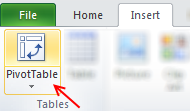
53 people said they love Pivot tables. They save you a ton of time, let you create complex reports, charts & calculations all with few clicks. No wonder so many people love them.

Pivot tables are ideal tools for managers & analysts who always have to answer questions like,

  • What is the trend of sales in last 6 months?
  • Who are our top 10 customers?
  • Which button do I press for strong latte?

May be not the last one, but Pivot tables can answer almost any business question if you throw right data at them.

Resources to learn Pivot tables:

4. Lookup Formulas

25 people said lookup formulas (VLOOKUP, HLOOKUP, INDEX, MATCH etc.) are their favorite feature of Excel. Lookup formulas help you locate any information in your workbooks based on input criteria. By knowing how to write lookup formulas, you can build dashboards, make interactive charts, create effective models & feel pretty darn awesome.

Resources to learn lookup formulas:

5. Excel Charts

Excel charts help you communicate insights & information with ease. By choosing your charts wisely and formatting them cleanly, you can convey a lot. I guess, most people hate Excel charts (hence it is at 5th position), because they are hard to work with. You can loose a whole afternoon formatting the wedges of a pie chart. But thanks to resources like Chandoo.org, you know better to make a column / bar chart and be done in 5 minutes.

Resources to learn Excel charts:

6. Sorting & Filtering data

If Microsoft ever needs few extra billions of cash, they just have to turn sorting & filtering features in Excel to pay-per-use. These ad-hoc analysis features are so powerful & simple that any aspiring analyst must be fully aware of them.

Resources to learn sorting & filtering features:

7. Conditional formatting

Conditional formatting is a hidden feature in Excel that can make your workbooks sexy. Just add some CF to highlight your data and you will turn boring into interesting. With new features like data bars, color scales & icon sets, conditional formatting is even more powerful.

Resources to learn conditional formatting:

8. Drop down validation & form controls

In-cell drop down boxes to collect user inputs - created using data validationRight from my 3.5 years old daughter to CEO of a company, Everyone loves to be in control. So how can you make your workbooks interactive, so that end users can control the inputs ?

By using form controls & drop down lists of course.

Resources to learn dropdown lists, form controls:

9. Excel Tables & Structural References

Introduction to Excel tables, what are they and how to use them?Excel tables, a new feature added in Excel 2007 is a very powerful way to structure, maintain & use tabular data – the bread and butter of any data analysis situation. With tables, you can add or remove data, set up structural references, connect them to external sources (SQL server, ODBC etc.), add them to data models (Excel 2013 onwards), link them to PowerPivot (Excel 2010 onwards), format automatically, filter & sort with ease and still be out of office before lunch break. It is a pity Microsoft did not call them pixie dust or magic mix.

Resources to learn Excel tables:

10. PowerPivot, Data Explorer & Data Analysis features

PowerPivot - Introduction, what is it and how to use it?Although Excel in itself is quite powerful, it struggles to analyze certain types of data,

  • Combining multiple tables and creating reports from them
  • Processing data from difference sources and getting output to Excel
  • What if analysis, scenarios & optimization

This is where add-ins like PowerPivot, Data Explorer and Analysis toolpak come in to picture. They let Excel do more, just like bat-mobile lets batman kick more ass.

Resources to learn more:

Learn all these features & more in one place

If you are looking to master all these top 10 features (and more) in one place, I highly recommend enrolling in my online classes. These training programs offer a step-by-step, in-depth, practical instruction on all areas of Excel, VBA, Dashboards & PowerPivot so that you can be awesome at your work. Click on below links to learn more.

Or if you prefer face-to-face training & live in USA, you are in awesome luck. I am visiting USA this summer to conduct advanced excel & dashboards masterclasses in Chicago, New York, Washington DC & Columbus OH.

Click here for details & to book your spot.


Facebook
Twitter
LinkedIn

Share this tip with your colleagues

Excel and Power BI tips - Chandoo.org Newsletter

Get FREE Excel + Power BI Tips

Simple, fun and useful emails, once per week.

Learn & be awesome.

Welcome to Chandoo.org

Thank you so much for visiting. My aim is to make you awesome in Excel & Power BI. I do this by sharing videos, tips, examples and downloads on this website. There are more than 1,000 pages with all things Excel, Power BI, Dashboards & VBA here. Go ahead and spend few minutes to be AWESOME.

Read my storyFREE Excel tips book

Overall I learned a lot and I thought you did a great job of explaining how to do things. This will definitely elevate my reporting in the future.
Rebekah S
Reporting Analyst
Excel formula list - 100+ examples and howto guide for you

From simple to complex, there is a formula for every occasion. Check out the list now.

Calendars, invoices, trackers and much more. All free, fun and fantastic.

Advanced Pivot Table tricks

Power Query, Data model, DAX, Filters, Slicers, Conditional formats and beautiful charts. It's all here.

Still on fence about Power BI? In this getting started guide, learn what is Power BI, how to get it and how to create your first report from scratch.

129 Responses to “Write a formula to check few cells have same value [homework]”

  1. Arie says:

    =NOT(STDEV(A1:A4))

    this also works for large ranges of numerical values (but not for text)

  2. Detlef says:

    Hi

    Works for numbers, text and logical values on a range from A1:An.

    =COUNTIF(A1:An,A1)=ROWS(A1:An)

  3. lockdalf says:

    well if you name the range, you could use following:

    =IF(SUMPRODUCT(1/COUNTIF('range','range'))=1,1,0) 

  4. Chris says:

    My solution is a, perhaphs slightly complex, array formula as follows:

    {=IFERROR(AVERAGE(IF(ISBLANK(A1:H1),9999,SUBSTITUTE(A1:H1,A1,9999)*1))=9999,FALSE)}

    Assuming there is a value (numerical, text, logic etc) in cell A1, this formula will work - and it will 'ignore' any cells that are 'blank' within the range A1:H1 (which can be extended to the required size).

    Breaking the formula down, the SUBSTITUTE(A1:H1,A1,9999) replaces all values (be it text / numerical) in the range A1:H1 that MATCH the value of cell A1 with the number 9999 (this should be changed to any number that WON'T APPEAR IN THE RANGE).

    These values are then multiplied by 1 (as SUBSTITUTE results in a text answer).

    Wrapping this in an IF(ISBLANK(A1:H1),9999,.........) formula takes care of any blank cells, setting them to this default value of 9999 also - this allows you to set the formula up once for a large range and then not have to alter as more data comes in.

    An Average is then taken of all these values - if all cells that contain values are the same, the average will come back to 9999.

    If all values are numerical but some differ, the average will differ from 9999 and will result in a FALSE answer. If some / all of the values are text and some differ from that in cell A1, the AVERAGE function will result in an Error, but in these instances the Match needs to return FALSE, hence the IFERROR function.

    Sure there's a simpler way to do this though!!

  5. George says:

    `{=IF(AND(COUNTA(RANGE)-SUM(--ISNUMBER(FIND(UPPER(FIRST ELEMENT IN RANGE),UPPER(RANGE))))=0,LEN(FIRST ELEMENT IN RANGE)=MAX(LEN(RANGE))),TRUE,FALSE)}`
    so if your data was in Column 1 and began in A1, you'd use
    `{=IF(AND(COUNTA($1:$1)-SUM(--ISNUMBER(FIND(UPPER($A$1),UPPER($1:$1))))=0,LEN($A$1)=MAX(LEN($1:$1))),TRUE,FALSE)}`

    This will work for strings and things, if you want it to be case sensitive (I don't), just remove the UPPER() part.
    What this does:

    `COUNTA($1:$1)`
    tells you how many entries you're looking at over your range (so we can work with an undetermined size).
    `--ISNUMBER()`
    ISNUMBER will return TRUE or FALSE depending on if the value inside is a number or not.  the -- part converts TRUE/FALSE in to 1 or 0.
    `UPPER()` OPTIONAL
    converts the value in to upper case.  If passed a number it changes it to text format.  This is what stops it from being case sensitive.
    `FIND($A$1,$1:$1)`
    will return a number if A1 is contained in each cell containing an entry in column 1.
    `LEN($A$1)=MAX(LEN($1:$1)`
    checks that all elements are the same length.  This is needed to avoid partial matches (without it, if A1 contained zzz and A2 contained azzza it would flag as true).

    REMEMBER this is an array formula, so enter with ctrl+shift+enter.

  6. Udit says:

    {=MIN(--(A1=OFFSET(A1,,,COUNTA(A1:A4))))}

    Gives 0 if false and 1 if true

  7. Ray Blake says:

    =COUNTIF(A:A,A1)/COUNTA(A:A) = 1

    This meets both bonus requirements and is dynamic. Keep adding more contents in column A and it will include these automatically. 

    • Mike K says:

      I like this a one a lot. I would make one small change by inserting a table for my data range. Makes it dynamic without selecting the whole column

       =IF(COUNTIF(tableName[colName],A2)/COUNTA(tableName[colName])=1,TRUE,FALSE)

  8. Sudhir Gawade says:

    For only Numeric values

    =MAX(A:A)=MIN(A:A)

  9. Sandy Siegel says:

    =(A1=B1)*(B1=C1)*(C1=D1)

  10. Elias says:

    Case sensitive.

    =SUMPRODUCT(0+EXACT(A1:A4,A1))=COUNTA(A1:A4)

    Regards

  11. PPH says:

    I'd use this

    =COUNTIF(range,INDEX(range,MODE(MATCH(range,range,0))))=COUNTA(range)

    It takes Hui's formula but ensures that the test value for the countif is the value or string that is most common in the range. Just in case you get a false but the problem is just with your test value being the odd one out.

  12. José Lôbo says:

    =SE(E(A1=A2;A1=A3);SE(E(A1=A4;A2=A3);SE(E(A2=A4;A3=A4);"ok")))
     
    SE = IF
    E = AND

  13. Stan Cullerne-Bown says:

    Bonus question 1 & 2
    Array formula: {AND(A1=A1:AN)}
    This will test all cells in range, including text and numbers. 

    Cheers 

  14. D Stinson says:

    A very simple solution uses Excel's Rank function.  Insert in B1 = Rank(A1, $A$1:$A$4).  Copy down this formula to B4.  If the answers in B1 thru B4 are all 1, the values are equal.  For an open range of cells, label the range of input (example "TestData") and place the label in the funtion (= Rank(A1, TestData) then copy down to an equivelent length of rows as the range.

  15. Tom Moedl says:

    =IF(SUM(A1:A4)/COUNT(A1:A4)=A1,TRUE,FALSE)

  16. Melanie says:

    =IF(SUM(A1:D1)/4=A1,"True","False")

  17. Tom Moedl says:

    I enjoy your emails.  I have learned a lot from them.  Thank you for what you do.

  18. .
     
    {=PRODUCT(--(A1=A1:A4))}
     
    .
    Change A4 to An.

  19. jimmy says:

    =IF((SUM(A1:A4)/COUNT(A1:A4))=A1,"TRUE","FALSE")

  20. Kishore Kumar says:

    I would use the formula which is mentioned below:-

    =IF(PRODUCT($A:$A)=A1^(COUNTIF($A:$A,A1)),"Yes","No")

  21. Karl says:

    At last a homework assignment that I could answer on my own. And I even understand some of the elegant answers from other readers this time.
    My solution was to nest IF statements:
    =IF(A4=A3,IF(A3=A2,IF(A2=A1,TRUE,FALSE),FALSE),FALSE)
    This satisfies bonus question 2 but I think the structure makes it impossible to modify this solution to satisfy bonus question 1. And I wouldn't want to use this strategy to compare very many values...

  22. Bob Bonner says:

    This answers all of your questions:

    =PRODUCT(--(INDIRECT("$A$1:$A$"&$B$1)=$A$1))

    where column A contains the values and $B$1 has the number of rows to assign to last A-cell. 

  23. Sanjay says:

    =IF(A1=A2:A2=A3:A3=A4>1,"TRUE","FALSE")
    =IF(A1=A2:A2=A3:A3=An>1,"TRUE","FALSE")
    =SUM(HELLO, A1)

  24. Livigs says:

    {=IF(SUM(IF(A1:A4=A1,0,1))=0,TRUE,FALSE)}
     
    This will work for numbers or text, and will work for any number of cells (A4 would just be An)

  25. Brian LaGrand says:

    Here's another alternate, assuming values in cells a1:d1
     
    =IF((A1*B1*C1*D1)^(1/COUNT(A1:D1))=AVERAGE(A1:D1),1,0)

  26. Supertaitai says:

    {=IF(AND($A$1:$A$4=OFFSET(A1,0,0)),1,0)}

  27. Virginia says:

    =SUM(IF(FREQUENCY(MATCH(A1:A4,A1:A4,0),MATCH(A1:A4,A1:A4,0))>0,1))

  28. Sanjay says:

    REVISED FORMULA
       =IF((A1=A2)*AND(A1=A3)*AND(A1=A4),"TRUE","FALSE")

    Regards

  29. Don says:

    =IF(SUMPRODUCT(--(A2:A5=A2))/COUNTA(A2:A5)=1,1,0)

  30. Bryan says:

    I would use something like this:  =COUNTA(A1:A4)=COUNTIF(A1:A4,A1)

    • Bryan says:

      You can even do a whole range and as you enter data into the range it tells you if they all match.  Going down to row 5000:  =COUNTA(A1:A5000)=COUNTIF(A1:A5000,A1).

      Thanks,
      B

  31. Manoj says:

    {=SUM(--(A1:A101=A1))=(COUNTA(A1:A10)+COUNTBLANK(A1:A10))}

  32. Ken ?-del says:

    For numeric values:

    =(OFFSET(list,,,1,1)=AVERAGE(list))

    where list = A1:A4 

    • Ken says:

      I need to retract my own post here guys. 

      It is WRONG! Let me explain.

      Suppose we have

      A1 = 1
      A2 = 0
      A3 = 2

      then Average = 1 and OFFSET(list,,,1,1) = 1
      so 1 = 1 but all the elements are NOT equal.


  33. Manoj says:

    correction 
    {=SUM(--(A1:A10=A1))=(COUNTA(A1:A10)+COUNTBLANK(A1:A10))}

  34. Pavel Lasák says:

    =IF(A1=B1,IF(B1=C1,IF(C1=D1,TRUE,FALSE),FALSE),FALSE) ....

  35. Matthew Holbrook says:

    =COUNTIF(OFFSET($A$1,0,0,COUNTA($A:$A),1),$A$1)=ROWS(OFFSET($A$1,0,0,COUNTA($A:$A),1))

  36. Parin Thacker says:

    I have a little more flexible approach. Suppose the value of 'n' is known. There is a possibility that only some of the cells in a row are filled up. For example if n = 10, then in a row, A1 to A10 must be compared. But in case only cells upto A7 are filled up. The formula thus has to adapt accordingly. Below formula does that:

    =COUNTIF(INDIRECT(ADDRESS(ROW(),1)&":"&ADDRESS(ROW(),COUNTA(A1:J1))),A1)=COUNTA(INDIRECT(ADDRESS(ROW(),1)&":"&ADDRESS(ROW(),COUNTA(A1:J1))))

  37. Ingo says:

    In A1:A100 is word/number
    In B1 is word/number we look

    C1=MAX(FREQUENCY(IF(A1:A100=B1,ROW(A1:A100)),IF(A1:A100<>B1,ROW(A1:A100))))  array formula

  38. Shubhro De says:

    We can use an array formula
    {=PRODUCT(--(A1:An=A1))}
    OR if we want n variable
    {=PRODUCT(--(INDIRECT("A1:A"&COUNTA(A:A))=A1))} 

  39. Steve LeLaurin says:

    {=AND(A1=A2:An)}

  40. Ariel says:

    I would use this one (simlpe)

    =(COUNTA(A:A)=COUNTIF(A:A;A1))

  41. uri Weiss says:

    try this
    =MAX(A1:A4)=MIN(A1:A4)

  42. uri Weiss says:

    Olso try this
    {=SUM(RANK(A1:A10,A1:A10))=COUNT(A1:A10)}
    Please notice it is an Array Formula

  43. elnur says:

    Dear All,
    i used that formula
    {=IF(COUNTIF(A1:A4,A1:A4)=COUNTA(A1:A4),TRUE,FALSE)}

  44. andy holaday says:

    Love the variety of responses.

    =MAX(A1:A4)=MIN(A1:A4)
    and
    =COUNTA(A1:A4)=COUNTIF(A1:A4,A1)
    will return true if the input range has blank cells

    My personal fave is the array formula {=AND(A1=A1:A4)}. Short and sweet, and easy to read. Blank cells will tally as a mismatch.

    A close second is 
    =SUMPRODUCT(1/COUNTIF(A1:A4,A1:A4))=1
    which will throw an error if blanks are present. 


  45. mahesh says:

    =PRODUCT(B1:D1)=B1^COUNT(B1:D1)...will return TRUE or FALSE

  46. Prem Singh says:

     
    Dear Sir,
     
    My answer is =exact(a2,a1)

  47. jack corley says:

    =IF((a1=a2=a3=a4),1,0)

  48. Arshad says:

    Hello Chandoo,
    We can also use Conditional Formatting......

  49. Akash Khandelwal says:

    For Numerics..

    =SUM(A1:AN)/A1=COUNT(A1:AN)
    results in True/False.

  50. Manoj Gupta says:

    =AND(IF(A1=B1,1,0),IF(B1=C1,1,0),IF(C1=D1,1,0))

  51. sam says:

    =AND(A1=A2:A4) array entered
    Generic
    =AND(A1=A2:An) array entered

  52. shrivallabha says:

    =--(COUNTIF(A1:A4,A1)=COUNTA(A1:A4))
    will give value as 1 or 0

  53. James says:

    Hi there, here's a simple formula to determine not only whether all 4 cells (A1 --> A4) are equal, but also whether any of the cells are equal and identifies which cells they are ...

    =COUNTIF($A$1:$A$4,A$1)*1000+COUNTIF($A$1:$A$4,A$2)*100+COUNTIF($A$1:$A$4,A$3)*10+COUNTIF($A$1:$A$4,A$4)*1

    A result of 1111 means no cells are equal, 4444 means all cells are equal, 1212 would mean there are 2 cells the same & they are in A2 & A4, etc

  54. Lood says:

    =((A1=B1)+(A1=C1)+(A1=D1))=3

    Obviously doesn't cover bonus question 1, but does so for q2 🙂
     

  55. Abhishek says:

    If formula

  56. Shmuel says:

    =MIN(A1:A4)=MAX(A1:A4)

  57. Faez says:

    Try this formula

    =IF(COUNTIF(A1:A4,A1)-ROWS(A1:A4)=0,"True","Flase")

  58. Werner says:

    I used the Swiss knife of excel: SUMPRODUCT, works for numeric as well as for non-numeric cell content and A1:A4 is obviously easily changed to any range.

    =IF(SUMPRODUCT(--(OFFSET($A$1:$A$4,0,0,ROWS($A$1:$A$4)-1,1)=OFFSET($A$1:$A$4,1,0,ROWS($A$1:$A$4)-1,1)))=ROWS($A$1:$A$4)-1,TRUE(),FALSE())

    • roirraWedorehT says:

      All of the individual non-array formulas (didn't test the array ones) have one flaw or another - mostly specifically if all the columns are blank, the result would still be false.

      Another formula in the comments worked for these but didn't work for when all columns had "0.00" in them. My solution was to OR the two. If H3 through H149 have your values, then this is what worked for me:

      =IF(OR(COUNTIF(H3:H149,H3)=COUNTA(H3:H149),SUMIFS(H3:H149,H3:H149,1)=COUNT(H3:H149)),IF(H3="","Blank",H3),"")

      This solution puts "Blank" if all the rows are blank, otherwise, it puts whatever the value that's in all of the rows - "0.00" or whatever.

      Thanks for all the answers!

  59. Allan R says:

    I used a nested if statement which also showed, via the false message, the first instance of cells which were not equal for the cells a1 to a5.

    =IF(A1=A2, IF(A2=A3, IF(A3=A4, IF(A4 = A5, "True","False A4"), "False A3"), "False A2"))

  60. Shailesh says:

    Hi,

    First, let me begin by saying, I am a big fan of all your posts and read your emails, mostly on the same day as you send them. I have not replied as much as I wanted to.

    This is my first attempt at answering a question on your post

    I came up with a simple check which will test if all values in a range A1:An are same or not

    Assuming range you want to check is A1:A10,
    In Cell B1, insert the formula 

    =IF(COUNTIFS(A1:A10,A1)=COUNTA(A1:A10),"All cells are same","All cells are not same") 

    The idea I applied is counting total number of non-blank cells and then counting the number of cells which match cell A1. If these are same, then it means
    a) all cells have the same value! (All can be blank, then both counts will be zero)

    I am working on finding the range automatically 🙂

    Can extend this into VBA and use InputBox etc to generate some user interaction

    Thanks
    Shailesh 

  61. Chirag says:

    =IF(COUNTIF(A1:A4,A1)=COUNT(A1:A4),TRUE,FALSE)

  62. Rafaqat Ali says:

    For homework & Bonus Question 3

    =IF(AND(A1=A2,A2=A3,A3=A4),1,0)


  63. Christopher A says:

    =IF(SUMIFS(A12:A15,A12:A15,1)=COUNT(A12:A15),1,0)

  64. Sanjeev Sawal says:

    One possible solution could be =+IF(COUNTIF(A1:A4,A1)-COUNT(A1:A4)=0,1,0)
    where A1:A4 is data range which can be a dynamic range and the formula can be modified accordingly. 
    Rgds,
    Sanjeev Sawal

  65. I got the right result with this one:

    =IF(A1=B1;IF(C1=D1;IF(B1=C1;1;0);0);0) 

  66. SIVAKUMAR R says:

    =and(a1=a2,a1=a2,a1=a3)
     

  67. SIVAKUMAR R says:

    ANSWER FOR bONUS 1

    =MAX(A1:A10)-MIN(A1:A10) 

  68. VaraK says:

    =AND(A1:A3=A2:A4)..Confirm with Ctrl+Shift+Enter (As as array formula). Works well for Text values and large range of values as well.

  69. Istiyak says:

    suppose cells contain 2 values ==== Yes | no

    formula :
    1
    =counta(a1:a4)=countif(a1:a4,"yes")
    It will return True or False.

    2
    =IF((COUNTA(A1:A4)=COUNTIF(A1:A4,"yes")),"Same value","Mis-match")
    it will return Same Value OR Mis-match.

    Hope you like it.

    Regards
    Istiyak

  70. Suraj Nair says:

    Also can use this formula
    =IF(AND(A1=A2,A1=A3,A1=A4),"1","0")

  71. Antonio says:

    Let say the values are in the range $B$1:$E$1, then the formula is:

    If(sumproduct(--($B$1:$E$1=$B$1))=CountA($B$1:$E$1);1;0)

    Please check that:
    * $B$1 was used as pivot value and could be randomly selected
    * It works well if parenthesis is omitted for values "1" and "0"
    * This formula applies also to "n-values" and non-numeric values (text, logical, etc.)

    Regards,

  72. Jorrie says:

    Hi, first time trying to solve a probleme.
    New at this but really enjoying Chardoo.org

    Think the following will work in all 3 questions

    {=IF(SUM(IF(A1=$A:$A,1,0))=COUNTA($A:$A),TRUE,FALSE)}

    Regards

    Jorrie
         

  73. Ashok Variyani says:

    use below formula for to get True / False

    =COUNTA(A1:A4)=COUNT(A1:A4)

    and use below formula for to get {1/0} or {match / Mismatch}

    =IF(COUNTA(A1:A4)=COUNT(A1:A4),{1,0} or {match,Mismatch})

  74. [...] Last week in Write a formula to check few cells have same value [Homework], [...]

  75. Cristian says:

    Hi, sorry if it's repeated, this array formula works well with numbers or text, the range can easily be dynamic: {=AND(A1:An=A1)} Now, after three days, I understand a lot more about array formulae, thanks?

  76. Adam says:

    =IF(AND(A1=A2,A2=A3,A3=A4),"TRUE","FALSE")

    • Yani says:

      What if there are not only four cells to compare but An?
      how will I determine if there is one cell that is not equal from any other cells?

  77. Netaji Bhopale says:

    =IF(COUNTA(A1:A4)=COUNT(A1:A4),1,0)
    =IF(COUNTA(A1:A4)=COUNT(A1:A4),”Match”,”Mismatch”)+
    =IF(AND(A1=A2,A2=A3,A3=A4),”TRUE”,”FALSE”)

  78. Aniket says:

    =iF(AND(EXACT(C15,D15),EXACT(E15,F15)),"Match","Mis-match")

  79. frank says:

    how this formula works in excel (B4+E4)/50*20
     

  80. Jerome says:

    I'm a little late to the party, but I figured I'd post anyways.

    For numbers only:
    =NOT(VAR.P(A1:An)) 

  81. nazmul_muneer says:

    The formula given below will fulfill the all criteria including bonus questions

    =IF(COUNTA(A:A)=COUNTIF(A:A,A1),"True","False")

    REGARDS 

  82. venkat says:

    =IF(MATCH(A1,A2:A4,0),TRUE,FALSE)
     

  83. Naveen Kumar says:

    =IF(COUNTIF($A$1:$A$4,A1)>1,"true","false")
    =IF(COUNTIF(A:A,A1)>1,"true","false")
     

    • Hui... says:

      @Naveen
       
      You can simplify your formulas as below:
      =COUNTIF($A$1:$A$4,A1)>1
      =COUNTIF(A:A,A1)>1
      Excel will return True or False without the need for the If() function

  84. Raghavendra says:

    Hi ,
     
    This question is similar to the one in the post.
    I have Text values in cell A1 and A2. 
    If A1 = A2, update 10 in cell A3 , else 0.
    Is there any formula for this. I am new to VB and hence do not have much knowledge. Eager to learn!!
     
    Thanks in advance !!!

  85. sandeep sharma says:

    =AND(A1=A2,A1=A3,A1=A4)

  86. sandeep sharma says:

    also =IF(AND(A1:A4=A1),TRUE,FALSE)

  87. Akshay says:

    One can use "IF, AND" formula.

    =IF(AND(A1=A2,A2=A3,A3=A1),"True","False")

  88. Cards says:

    =COUNTIF(A:A,A1)=COUNTA(A:A)

  89. Ritesh says:

    Enter array formula like, = IF($B$16:$B$21=$B$17:$B$22,"Yes","No")

  90. sunil gupta says:

    =IF(AND($E$5=$E$6,$E$6=$E$7,$E$7=$E$8),"true","flase")
    it can work try this one

  91. Andy Gore says:

    A question for you
    sheet 1 table A1:C10

    What formula in sheet 2 A1 will give me what is entered in the table sheet 1 A1:C10
    There is usually only one entry made in the table but if you can supply the answer to 1 or 2 entries I would be grateful

  92. Duncan says:

    =max(A:A)=min(A:A)

  93. Eduardo says:

    FOR TEXT DATA
    =COUNTIF(A1:A5,a1)=COUNTIF(A1:A5,"*?")

    FOR VALUE DATA
    =COUNTIF(A1:A5,A1)=COUNTA(A1:A5)

    Both Return TRUE or FALSE

  94. kaushik says:

    =if({sum(1/countif($A$1:$A$n,A1:An)}=1,"All Same","Not All Same")

  95. manish gupta says:

    I use formula A1=B1 and get value of TRUE / FALSE in C1. I had dragged this formula for 10 rows. Now in cell D2 i tried to put formula..

    =if(and(c1="False", c2="true"), "conflict", "no conflict")

    but even when the condition is true i am still getting no conflict.

    Can you please advice?
    thanks,
    Manish

    • Hui... says:

      @Manish
      Remove the " from around True and False
      =if(and(c1=False, c2=True), "conflict", "no conflict")

      In C1 and C2 you have a Boolean expression and it evaluates as True/False
      These are not text, although they do appear as Text, they are not 1/0 although they sometimes behave as 1/0, they are in fact Boolean values True/False

      So in your example you can simplify it as
      =If( And( Not(C1), C2), "conflict", "no conflict")

  96. Mohammed says:

    =SUMPRODUCT(MATCH(A1:A4,A1:A4,0))=COUNTIF(A1:A4,A1)

  97. adivyom says:

    Answer to both bonus questions 2 and 3:

    =COUNTIF(A1:An,A1)=COUNT(A1:An)

  98. Yves S says:

    answer to all questions:
    ={IF(ISERROR(MATCH(FALSE,((A1:An)=$A$1),0)),"same","different")}

    this works with numeric, non-numeric, and blanks:

    COUNT will not count numeric
    COUNTA will count blanks as one

  99. cnestg8r says:

    =SUMPRODUCT(1/COUNTIF(B1:J1,B1:J1))

    This will tell you how many unique values exist in the selected range. Text or numeric mixed.

  100. RAJIV SIROHI says:

    {=IF(AND(A1:A9=A2:A10),"EQUAL","NOT EQUAL")}

    this is an array formula, insert it with CSE.

  101. Anonymous Coward says:

    COUNTA/UNIQUE

  102. Tiago Couto says:

    =SUMPRODUCT(A:A)/A1=COUNT(A:A)

  103. Gabe says:

    =COUNTIF(A1:A4,A1) = COUNTA(A1:A4)

Leave a Reply