
We are busy decorating the Christmas tree, making preparations for the holidays. But I have a very quick tip for you.
[Note: all these tips work in Excel 2007 or above]
Whenever you are working with huge lists of data, filtering & sorting is one simple way to analyze the data quickly.
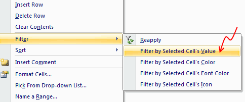
You can quickly filter your data based on current cell’s value by right clicking and then selecting filter > filter by selected cell’s value.
Bonus tips on Filters:
- You can even filter by selected cell’s color, font or conditional formatting icon.
- You can also sort a list by selected cell’s column in either ascending or descending order.
- You can instantly turn on / off filters by pressing CTRL+SHIFT+L


12 Responses
This works in Access too (even 2003), where you can right-click a value in a table and choose “Filter By Selection” to see only records matching that value.
That was actually a nice little tip I didn’t know existed, especially considering no filters are applied to the data before you generate the shortcut.
Very good tip! I did not know this one. It is a good reminder to explore the many options on the right-mouse click short menu.
I also did not know the Ctrl + Shift + L Keyboard shortcut. Thank you. I am going to share both of these tips with my readers at TheCompanyRocks.com. I am also adding your website to my Blog Roll.
Happy Holidays!
Danny Rocks
The Company Rocks
Yes, but when you CTRL+SHIFT+L it will erase your filter setting if you already have filters on the top row so it not worthwhile.
Great tip, but it does not work when Page Break Preview is active
Pivot is also a great tool to do your analysis, its much more powerful than filters
Pivot is a powerful tool for data display,
But pivot does not allow changes to the source data
Filter is a supreme tool for editing and altering the pivot ssource its self
i will most definitely stop using the sequence
for + +
Thanks
i will most definitely stop using the sequence ALT D F F and switch to Ctrl + Shift + L
This works, I tried it
http://answers.microsoft.com/en-us/mac/forum/macoffice2011-macexcel/filter-by-cell-value-shortcut/d5189f6a-7527-4768-a83b-ad3d4ff3ba74
Dears,
The ‘filter’ option in the right click menu is showing up in Excel 2007 only for table formats. Can we apply filter by selected cell on a simple sheet (not table)?
I posted this again just to be notified for any follow-up comments.
Thanks.