
 In October 2008, I have started an ambitious series of posts on this blog called – Spreadcheats. These are little tricks, nuggets, tutorials on using Excel that would make anyone a spreadsheet guru.
The spreadcheats series has been wildly successful. I am compiling all this useful information and articles in to one big post so that anyone can follow the links and become good in Excel. Read on,
[Note: This is not for beginners. If you know what a formula is, you would enjoy this 31 articles]
1: Insert Line Breaks in a Cell
Press ALT+Enter keys in a cell to make a new line inside the cell. [Read this]
2: Select all cells in a range
Use these keyboard shortcuts to select all the cells in a range or group. You can find 90 more shortcuts on that page. [Read this]
3: Using Mouse in Excel

Many of us know at few keyboard shortcuts. But what about mouse short-cuts? Read this post to learn interesting mouse shortcuts that can boost your productivity. [Read this]
4: Using Mouse in Excel – Part 2
In the second part of Mouse shortcuts, we explore double click tricks in Excel. [Read this]
5: Save time by using chart templates
In this spreadcheat, learn how to make your own chart templates and re-use them to save time. [Read this]
6: Make ToC (Table of Contents) in Excel – and other tricks
We all run in to large excel workbooks one time or other. Read this post to find out how you can manage when you have a large file. [Read this]
7: How to print spreadsheets one just one page?
Use the little trick in print settings to print any worksheet on just one page. [Read this]
8: Write better formulas by knowing the difference between relative and absolute references

Quick, what is the difference between A1 and $A$1? If you said 2 dollars, you are the right person to read this article. Learning the differences and usages of various reference types in Excel is important if you want to write better and simpler formulas. [Read this]
9: Remove duplicate items using formulas
Learn how to remove duplicates, identify unique values etc. using formulas in this article. [Read this]
10: Introduction to VLOOKUP Formula (and MATCH, OFFSET Formulas)
VLOOKUP remains one of the most important and very useful formulas in Excel. Learn how to write vlookup formulas by reading this article. [Read this]
11: Introduction to 3D References in Excel (a tutorial on Employee Satisfaction Surveys in Excel)
In this tutorial, we will explore a feature called 3D References in Excel and build an employee satisfaction survey form in Excel. [Read this]
12: Introduction to SUMPRODUCT formula
Learn how to use SUMPRODUCT to find sum of values that meet more than one condition. [Read this]
13: Introduction to ROWS and COLUMNS formulas
One of my recent favorites, ROWS() formula is very useful to generate sequential numbers in Excel. [Read this]
14: Calculate Moving Average in Excel
Use excel formulas and relative references to calculate moving average from your data. [Read this]
15: Introduction to FREQUENCY formula
We use FREQUENCY formula in Excel to generate statistical distribution of a set of values in this example. [Read this]
16: How to understand and fix excel formula errors
If you are ever perplexed by #N/A, #NAME! and said #$#@ to excel, this is the article for you. Read it to learn what these errors actually mean and how to fix them. [Read this]
17: Quick tip to Debug Complex Excel Formulas
Use Function key F9 to debug lengthy and complex excel formulas. Select a portion of the formula and press F9 to instantly evaluate that portion and see the result. Read this article to find out how to use this trick. [Read this]
18: Use Find / Replace tool to change formulas
Learn how to use Find / Replace tool in Excel to quickly edit formulas and change them. [Read this]
19: Introduction to COUNTIF and SUMIF Formulas
COUNTIF and SUMIF are very simple yet very powerful formula tools for anyone using Excel. In this article, explore these formulas and learn to use them. [Read this]
20: Introduction to Array Formulas in Excel
Array formula is like a mega formula that would work on an entire range of cells and return another range of cells. They are useful for scenarios where the output we need is not one value but a set of values. In this introductory example, learn how to write your first array formula. [Read this]
21: Introduction to Excel Conditional Formatting
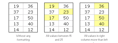
Excel conditional formatting is your way of telling excel to highlight / change formatting of cells that meet certain criteria. This is a good way to draw attention to few points from a large table. Learn how to use Excel CF in this introductory article. [Read this]
22: Introduction to Excel Camera Tool
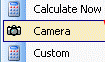
In this article, learn about Excel Camera (or Snapshot) tool which is useful for making a live snapshot of a range of cells. [Read this]
23: Introduction to Excel Pivot Tables
Pivot tables are a powerful way to analyze and report your data. In this introductory post, you will find all the basics of pivot tables and learn some tricks. [Read this]
24: Introduction to Excel Goal Seek
Goal Seek is opposite of formulas. In formulas we tell excel a bunch of values and excel finds the result. In goal seek, we tell excel what the result should and excel tells us what kind of parameters should be given. This is useful to find, for eg. Your retirement nest egg value … [Read this]
25: Introduction to Combination Charts in Excel
Learn how to combine 2 different chart types in to one chart in this article. [Read this]
26: Make a Dynamic / Interactive Chart using Data Filters
Do you know that we can use data filters to filter charts as well as data? Well, in this article, you can learn a powerful yet simple trick to make a dynamic chart in Excel using data filters alone. [Read this]
27: Make a Dynamic / Interactive Chart using INDEX Formula
Learn how to set up a dynamic or interactive chart using INDEX formula and Camera tool in Excel. [Read this]
28: Make Collapsible Charts using Group – Outline Tools
We can collapse / expand charts using the group and outline tools in Excel. Learn how to set up such a collapsible chart in Excel. [Read this]
29: Showing Chart Labels in Different Colors – Charting Tricks
Learn how to use custom cell formatting codes to show chart labels in different colors based on a criteria. [Read this]
30: Advanced Data Validation Tricks in Excel – Part 1
In part 1 of excel data validation tricks, we will learn how to use excel formulas to control the way data validation works. [Read this]
31: Advanced Data Validation Tricks in Excel – Part 2
In part 2 of data validation tricks, we will learn how to prevent duplicate data entry using data validation formulas. [Read this]
Happy learning 🙂


19 Responses to “31 Excel Tutorials – Learn and Be Awesome in Excel”
@Teylyn... Thanks for the comment. I have changed the post title to a more meaningful "31 Excel Tutorials - Learn and Be Awesome in Excel". I agree that original title was marketingy.
That was quick, Chandoo! Please feel free to delete my comment so as to avoid confusion in your subscribed audience.
My subsription will not be cancelled any time soon!
cheers
teylyn
@teylyn: Get a life, man.
The best tricks for using Excel I've ever found have been on this blog. Everyone in my office devours every post he makes. The use of the word "guru" is a non-issue: besides, it made you click through to the main article.
Your point about the marketing focus is made. However, when the plebes complain too much, the emperor takes away social services and starts murdering people in the Coliseum. Don't make the emperor angry.
sinfonian, you may note that the emperor actually agreed with my sentiment.
Chandoo, I think it's time to delete my first comment. 🙂
Social comments and analytics for this post...
This post was mentioned on Twitter by Excel_Insider: Become an Excel Guru in 31 Days: In October 2008, I have started an ambitious series of posts on this blog called... http://bit.ly/aZ5d44...
These are wonderful tips Chandoo! =)
@Teylyn and sinfonian0294: I must be fabulously lucky to have people like you in our community. Thank you 🙂
@Eric: Thanks ...
....Awesome excel tricks, but also awesome blog for the pleasure to read, the visual appeal (!) as well as the wording appeal (I loved you word "marketingy"(...!).On the marketingy side, even that is made in such a fun way, that all is appealing.
Hooked on the site, and definitely not going to let go!
Danièle
Your tips are really something to be appreciated!
I have a problem!!
I feel you are the guy for it!!!
Chandoo,,
UR d best!!!!!!!!!!!! Chandoo Rocks.!!!!!1
Tnakx budddy...
Chandoo,
LOVE this site; it has helped me so much, I am now beginning to be able to help others. Wish I could find the same no hinny biting, straight forward, approach for an Access blog. Well a girl can always dream 🙂
I laughed about sinfonian0294s, "Guru "remark. Monday when I passed on the link to this site to a co-worker, I described you as the Excel God. No offense intended.
Thank you for this blog and all the effort you put into it.
Trianna
@Trianna... Thanks for your love and support 🙂
Hi Chandoo
Firstly i really loved ur Websites on Excel Is Awesome, but i found some fault in some part. chandoo i think its important that u should get honest suggestion so that u can improve more on ur sites. The Thing i felt is that there are many link on the Excel Intermediars. I really want u to specify where exactly a begineers can start learning some Excel Lessons. There should be Excel Lessons on Excel Topics and then there should be link inside on that topic which specify depth knowledge so that a learner can learn from start and serially and also in depth. So point is just mention Excel Lessons from start and inside Links on particular topics with Example on particular Topic. then he can learn a lot. I hope u will get a look on my point. hope to see changes.
YEAH I HAVE COPY PASTED THE ABOVE COMMENT; SAME REQUEST HERE
Hi Chandoo
Firstly i really loved ur Websites on Excel Is Awesome, but i found some fault in some part. chandoo i think its important that u should get honest suggestion so that u can improve more on ur sites. The Thing i felt is that there are many link on the Excel Intermediars. I really want u to specify where exactly a begineers can start learning some Excel Lessons. There should be Excel Lessons on Excel Topics and then there should be link inside on that topic which specify depth knowledge so that a learner can learn from start and serially and also in depth. So point is just mention Excel Lessons from start and inside Links on particular topics with Example on particular Topic. then he can learn a lot. I hope u will get a look on my point. hope to see changes.
Chandoo,
Terrific site! You are my #1 source for knowledge checking on Excel!
Fazil
[...] 31 Excel Tutorials – Learn and Be Awesome in Excel | Pointy Haired Dilbert: Learn Excel Online ... says: March 11, 2010 at 1:00 pm [...]
I like http://best-excel-tutorial.com tutorial too. But yours is ouf course better 🙂
[…] your looking to further your Excel skills, I highly recommend you challenge yourself with this online tutorial put together by Chandoo.org – 31 Excel Tutorials – Learn and Be Awesome in […]