
Moving average is frequently used to understand underlying trends and helps in forecasting. MACD or moving average convergence / divergence is probably the most used technical analysis tools in stock trading. It is fairly common in several businesses to use moving average of 3 month sales to understand how the trend is.
Today we will learn how you can calculate moving average and how average of latest 3 months can be calculated using excel formulas.
Calculate Moving Average
To calculate moving average, all you need is the good old AVERAGE excel function.
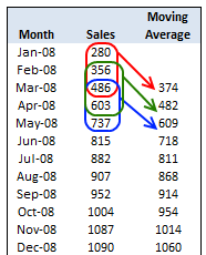
Assuming your data is in the range B1:B12,
- Just enter this formula in the cell D3
- =AVERAGE(B1:B3)
- And now copy the formula from D3 to the range D4 to D12 (remember, since you are calculating moving average of 3 months, you will only get 10 values; 12-3+1)
- That is all you need to calculate moving average.
Calculate Moving Average of Latest 3 Months Alone
Lets say you need to calculate the average of last 3 months at any point of time. That means when you enter the value for the next month, the average should be automatically adjusted.
We can do that using excel formulas AVERAGE, COUNT and OFFSET
First let us take a look at the formula and then we will understand how it works.
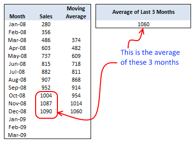
=AVERAGE(OFFSET(B4,COUNT(B4:B33)-3,0,3,1))
So what the heck the above formula is doing anyway?
- It is counting how many months are already entered – COUNT(B4:B33)
- Then it is offsetting count minus 3 cells from B4 and fetching 3 cells from there – OFFSET(B4,COUNT(B4:B33)-3,0,3,1). These are nothing but the latest 3 months.
- Finally it is passing this range to AVERAGE function to calculate the moving average of latest 3 months.
Your Home Work
Now that you have learned how to calculate moving average using Excel, here is your home work.
- Lets say you want the number of months used to calculate moving average to be configurable in the cell E1. ie when E1 is changed from 3 to 6, the moving average table should calculate moving average for 6 months at a time. How do you write the formulas then?
Don’t look at the comments, go and figure this out for yourself. If you cant find the answer, come back here and read the comments. Go!
This post is part of our Spreadcheats series, a 30 day online excel training program for office goers and spreadsheet users. Join today.


196 Responses
Hello, just recently found your website and I’m loving all the tips. Thank you for all your tutorials. It’s exactly I needed however, I ran into a bit a problem as I am also using Vlookup with Offset. For instance, in your example, I would use Vlookup in my template so that as I put in new data every month, it would automatically update the sales data each month.
=IF(ISBLANK(VLOOKUP($A15,Data,45,FALSE)),” “,(VLOOKUP($A15,Data,45,FALSE))).
My problem is in my OFFSET formula, I have COUNTA which obviously counts any cells with formulas, even ” “. Any ideas how to incorporate these two functions better, especially when I am trying to graph and average that last 12 months?
I would appreciate any ideas you or your readers my have. Thanks, again, for the the awesome site!
@Twee… welcome to PHD and thanks for asking a question. I am not sure if I understood it correctly though. Have you tried using count instead of counta?
You havent shown us the offset formula, without looking that fixing it would be difficult…
I did the home work that is calculate the moving average for 6 moths alone and I got the following number using this formula. Please can you let me know if this correct and also if there are alternative methods to answer the homework.
Thank you
“=AVERAGE(OFFSET(C36,COUNT(C36:C47)-6,0,6,1))
Result 987
=AVERAGE(OFFSET(B1,(COUNT(B:B)-E1),0,E1,1))
Good work out for my foggy brains.
not a perfect answer! only conceptually correct.
=IF(COUNT($A$5:A7)>=$B$2,AVERAGE(OFFSET($A$5,COUNT($A$5:A7)-$B$2,0,$B$2,1)), “”)
where
B2 contains my Moving Average number
my data lies in cells a5 through a22
Chandoo, my first post ever. Nice job with your site though. totally awesome
Hi Chandoo – coincidentally I did a post on moving averages as well recently:
http://newtonexcelbach.wordpress.com/2009/04/25/moving-averages-and-user-defined-array-functions/
You’ll have to wait for the next post to find out why I used a UDF, rather than the built-in average function 🙂
Hi Chandoo,
Thank you for suggesting I use Count instead of Counta. I don’t know I was so stuck on counta and didn’t think of count instead!! I just tried it and it worked beautifully!! Oy!! Something so simple and I was stuck on it! Thanks, again, for the tutorial on OFFSET because it’s indeed powerful!
@Paresh, IndianJewel: Thanks for sharing 2 very good ways to do this.
Learning to offset is very critical when you are working with ranges of varied (and unknown) sizes.
@Doug: I have seen your post in google reader after scheduling this, otherwise I would have linked to it from this post itself… Thanks for sharing the URL.
@Twee… you are welcome 🙂 I am happy you could solve this…
Hey guys,
Can someone help me to figure out how to calculate the average based on a 365-day rolling average.
I do have up to 6 month of daily data and keep collecting them and would like to know what would be the 365-rolling average.
Assume you data is in B2 to B366 then using
=SUM(B2:B366)/COUNT(B2:B366)
Is this a right way to do it. Or use this formula
=SUM(B2:B366)
then =B2/365
I don’t get the same results and need to know which one is right and why?
Can someone out there help me?
Thanks,
ForMcmurray
Sorry I had to fix my formula…
Hey guys,
Can someone help me to figure out how to calculate the average based on a 365-day rolling average.
I do have up to 6 month of daily data and keep collecting them and would like to know what would be the 365-rolling average.
Assume you data is in B2 to B366 then using
=SUM(B2:B366)/COUNT(B2:B366)
Is this a right way to do it. Or use this formula
=SUM(B2:B366) result goes to C2
then =C2/365
I don’t get the same results and need to know which one is right and why?
Can someone out there help me?
Thanks,
ForMcmurray
@FortMcmurray: Welcome to PHD and thanks for asking a question. The reason why you are seeing different results is because your data might have zero / blank elements. When calculating averages often you may want to omit zero / blank values. Also, instead of using sum()/count(), you may want to try the average() formula. You can learn more about average formula here: http://chandoo.org/excel-formulas/average.html
As long as you have values in all the cells, all sum()/count(), sum()/365, average() should return the same value.
Thanks Chandoo for your help. But how do you address situation where you do not have a whole year data but nonetheless you are trying to calculate the moving average based on a 365-day?
Do you put zero for those cell that you don’t have value or leave them blank?
@FortMcmurray: The point of moving average is, it is calculated for a moving window of values. So when you have values less than a year, you cannot calculate moving average. Whenever we calculate moving average of n values over a range of M values (n<M), you get M-n+1 moving averages.
Hi,
I am trying to calculate 30 days rolling data . Can any one help me out here. I have 30 days figure. and going from 1st of the next month I want my data to be automatically picked up on 30 days rolling period. Any one help here will be highly appreciated.
@Amber, you can calculate this very easily. Assuming you have data in the range A1:A1000, in B30, you can write the formula average(a1:a30) and then copy the formula down.
hello..,
can you help me to calculate the sales of Jan 09,Feb 09,Mar 09 ..ect.using this formula..in the above example ?
@Shamsuddin.. you mean calculating sales values from the moving average?
HELP!! i am new at excel and i need to find the average YTD over 12 months. each month has its own month total on an individual worksheet. what would the formula be?
@Cordell.. is the value for month-wise total in the same cell in individual sheets? If so, you can use 3d References to solve this… like,
=AVERAGE(JAN09:DEC09!A1)
(assuming sheet names are JAN09, FEB09… DEC09 in that order)
You are THE MAN
thank you for this website
God Bless
have a question here:
i have measurements performed every 10 minutes for a longer period (few months)
i want to calculate daily averages without having to select all data the needs to go into these averages
can anyone help
thanks
A.
@Alejandro… assuming you have measurement date-time in column A and measurement in column B,
You can get daily averages like this:
List down the dates for which you need daily averages in column C.
In column D, write a formula like this: =sumproduct(–(int($a$1:$a$100)=c1),($b$1:$b$100))/sumproduct(–(int($a$1:$a$100)=c1))
change the range values as you please. For more on sumproduct formula visit – http://chandoo.org/wp/2009/11/10/excel-sumproduct-formula/
Chandoo,
I have a large database with several columns of data over 3 years. I am trying to build a formula at the end that will take rolling average of the last 30 pieces of data. I understand your formula all the way until you get to the end what is the 0,3,1 mean? Does this stay the same for all applications?
=AVERAGE(OFFSET(B4,COUNT(B4:B33)-3,0,3,1))
Chandoo,
I have several columns that have information in them. I am trying to create a last thirty pieces of data moving average. Each time I add data I want it automatically update the moving average. The problem I have is that I have some columns that have sporatic data in them and when I apply the above formula It is not taking the last 30 pieces of data. If I have 3 blank cells in the column it is taking the average of the last 33 pieces of data. Is there a way to only have it look at cells with data in them and count the last entered data backward 30 to calculate the moving average? Below is the formula I have entered. Any thoughts? (G4 is the start of the data in the column) (G4:G314 is the range of data)
=AVERAGE(OFFSET(G4,COUNT(G4:G314)-30,0,30,1))
@Geoff… sorry for responding late. I forgot your comment until today.
For OFFSET help pls visit http://chandoo.org/wp/2008/11/19/vlookup-match-and-offset-explained-in-plain-english-spreadcheats/ and see the examples. You should be able to make sense of them.
Coming to your problem regarding blanks and sporadic data, here is how I would solve it.
Insert a new column next to column G where you have the data. Write “1” in first cell. In the subsequent cells write =IF(G5=””,H4,H4+1)
This will show numbers in incremental order but shows same numbers when the value in column G is a blank. Paste this formula in the range H5:H314.
Now, the moving average formula becomes =AVERAGE(OFFSET(G4,MATCH(MAX(H4:H314)-30+1,G4:G314,0),0,
MATCH(MAX(H4:H314),G4:G314,0)-MATCH(MAX(H4:H314)-30+1,G4:G314,0)+1
,1))
Essentially we have introduced a new column and are using MATCH to find the position of 30 th cell from last with a value in the range G4:G314. Once we know the position of it (MATCH(MAX(H4:H314)-30+1,G4:G314,0)) , we just offset the range from that point MATCH(MAX(H4:H314),G4:G314,0)-MATCH(MAX(H4:H314)-30+1,G4:G314,0)+1 cells.
I am going to write another tutorial on this problem as it is quite interesting. You can get a downloadble file then. Meanwhile you can try these formulas. You seem like you already know what to do, so this should help you get going.
I realize the formulas are kind of messed up. This is how it should have read.
—
Now, the moving average formula becomes =AVERAGE(OFFSET(G4,MATCH(MAX(H4:H314)-30+1,G4:G314,0),0,
MATCH(MAX(H4:H314),G4:G314,0)
-MATCH(MAX(H4:H314)-30+1,G4:G314,0)+1
,1))
—
I need to calculate a 12-month rolling average that will encompass a 24 month period when completed. Can you point me in the right direction as too how to get started? My data is vehivle miles and starts on B2 and ends on B25. Help!!
Bigdog
Chandoo, this is a great formula for what I am using except I am trying unsuccessfully to make the formula conditional. I have a spreadsheet, see links below, that tracks all rounds of disc golf played by friends and myself.
http://thegrammatoncleric.com/DiscGolfTracker.htm
http://thegrammatoncleric.com/DiscGolfTracker.xls
I’ve already got it setup to calculate each of our overall averages and each of our averages on specific courses. What I am trying to do now however is also setup a moving average based off our 5 most recent rounds. Once more data has been entered I will change it to 10, but for now 5 will be just fine. I can get the moving average to work, but I cannot figure out how to add conditional restrictions. IE I want for example just the last 5 rounds that were played by Kevin. After that I will want just the last 5 rounds played by Kevin at the Oshtemo course.
The code I’m using is below.
Code for Cell C9 is listed below.
=IF($B9=0,””,IF($B9<6,AVERAGEIF(DiscRounds!$A$2:$A$20000,$A9,DiscRounds!$M$2:$M$20000),AVERAGE(OF FSET(DiscRounds!$M$2,IF(DiscRounds!$A$2:$A$20000=$A9,COUNT(DiscRounds!$M$2:$M$20000),"")-5,0,5,1))))
Essentially if there are 0 rounds it leaves the cell blank. If there are 5 or fewer rounds it just uses the average of all rounds. Finally, if there are 6 or more rounds the code then uses your AVERAGE function from this post. After trying many things however I am uncertain how to conditionally pull the last 5 rounds so that it only pulls the last 5 rounds of the individual named in cell $A9.
The formula I am referencing is NOT currently in cell C9 on my spreadsheet that is linked. I just have been testing it there.
@DND: use the following formula in cell C13 onwards =AVERAGE(B2:B13) and drag down.
@TGCRequiem: If you have excel 2007, you can use the AVERAGEIFS formula to achieve this.
Hi Chandoo, You can use negative numbers in offset for rows/cols/height/width. So instead of doing -3 in rows and then +3 in height, you could just do it at once as -3 in the height. 🙂
Surprised that no one (out of close to 10K readers) pointed that yet on this year old article of yours!!
@Vipul… Since writing this article I have realized that we can use negative numbers in OFFSET. I will probably include this idea in an upcoming tutorial.
Be not surprised that nobody uses negative height. Microsoft Help on the Offset function explicitly states that Height and Width must be positive numbers. What is surprising is that users trust that MS Help is always correct. Which it certainly is not.
Regards
Brian
I need to calculate a 12-month rolling average to roll up into a separate summary sheet. My monthly data is entered (and will be entered) in cells B4 thru B26 of sheet 2, and there are some blank cells for future entries. (Each month, I enter data on the next available row). I need to calculate the average of the last 12 months (entries) in that column and have that figure entered on cell C4 of Sheet 1. Can you help me?
@Pap… Use the formula =average(offset(Sheet2!b4,counta(Sheet2!B4:B26)-12,0,12,1))
Hi all,
Just adapted this to fit the data I was working on after going through a few interpretations. This is a fantastic site and a great explanation. Thanks for the big help Chandoo!
As a heads-up to other users to help them save time if they are doing something similar I was working with stock data in the format; date (A:A), open(B:B), high(C:C), low(D:D), close(E:E) and fitted the formula in the following order (copied from cell H:15):
=AVERAGE(OFFSET($E$2,COUNT($E$2:E15)-$H$3,0,$H$3,1))
where $H$3 is the reference cell that determines the length of the moving average lookback period.
Hello,
I was just wondering if you could use the offset function within a pivot (calculated field)?
If so, how would that be done?
Many thanks – Your site is gem!!!
Tracey
Hi
This discussion I have found very helpful and I have solved a moving average problem adapting the formula mentioned above =AVERAGE(OFFSET(G4,COUNT(G4:G314)-30,0,30,1))
by Geoff.
However I notice this works when cells contain data, but if a cell has a 0 value this will be included in the average calculation unless those 0 values are removed . Is there a way to write the same formula but include something to exclude (not hide) any cells containing a 0 value?
@Tracey… I do not think you can use OFFSET in Pivot calculated fields.
@Eoin: You can modify the formula to omit zeros like this:
=SUM(OFFSET(G4,COUNT(G4:G314)-30,0,30,1))/ COUNTIF(OFFSET(G4,COUNT(G4:G314)-30,0,30,1),"<>0")PS: I have not tested it, but it should work without too much tweaking.
Thanks very much, this works fine and gives a truer average.
Eoin
Hello Chandoo,
I am strugling with Pivot table trying to compile in a field the moving average (on last six month values) of another field.
Have you any idea on how top proceed?
thanks
This works great, except I always get an error that says “The formula in this cell refers to a range that has additional numbers adjacent to it.” I have to manually click on “Update formula to include cells”, how can I have this done automatically? Thanks in advance
Lawrence
@Snooo: I am not sure if you can do moving averages in pivot tables natively. But you can do this by adding extra calculation right next to pivot table.
Assuming your pivot’s values start from B5 (that is B5 is the first cell to have a value other than labels)
In any free cell write =AVERAGE(OFFSET(B5,COUNTA(B:B)-COUNTA(B1:B5)-6,0,6,1))
This will get you the average of last 6 values in the pivot (assuming you dont have totals / grand totals on)
@Lawrence: Since we are referring only 3 cells (or 4 or 5 etc.) at a time, you might get this error. You can turn off this notification by going to excel options > formulas and then unchecking the box that says “formula omits cells in adjacent region”.
Chandoo,
thanks for this workaround, I already applied it following your hints on the previous posts of this page. The point is that is not as flexible as a field in a Pivot Table.
If you discover an alternate Pivot-native solution for moving-averages, do not hesitate to propose it.
thanks again.
I am trying to have a rolling 56 day window of data. I don’t need an average but rather the count and was trying to use countif function to count how many samples in the 56 day window were positive.
Is there any way to use count instead of average?
@Stefanie… Welcome to chandoo.org
You can do that like this:
Assuming your data is in column A, from cell A2:A301. And you want to findout how many positive values are there in each of the 56 values starting A2.
in B2 write =Countif(a2:a57,”>0″)
Now drag B2 thru B301 to auto fill.
We have two data results put in daily and would like to see our rolling window for every 56 days. I have done the countif function previously, and can get the 56 day results for that current window, if i plug that in everyday. We want a function so that it can be a rolling window and as we go to the next day the information will change. I know I can drag down to get that day’s currents 56 day window, but was hoping there was a way to only have the most recent information showing and not everyday’s.
I have a whole sheet of information on one sheet and then on another “results” tab I am trying to break down the information in the current 56 day window.
@Stefanie
Have you tried Pivot Tables, which can summarise data easily
Do you always have 2 entries per day?
Do you ever have any days with 1 or 3 entries ?
What Columns is your Data and Dates in ?
I haven’t tried Pivot Tables and haven’t done too much work previously with them. The Date is in column A and the Result for the test (Pos. or Neg.) is in column F. And there are only two samples everyday.
@Stefanie
If the first row of a date is in an even row try in
A2: =IF(ISEVEN(ROW()),COUNTIF(F2:F115,”>0″),””)
or Odd Row try in
A3: =IF(ISODD(ROW()),COUNTIF(F2:F115,”>0″),””)
and copy either down
or a bit more flexible
A2: =SUMPRODUCT(($A$2:$A$300>=A2)*($A$2:$A$300<=A2+56),($F$2:$F$3000))
Hey man – thanks for the site – this is the only rolling average calculation that I have actually gotten to work. One question though – what modifications are needed if the data are arranged horizontally – if I use this formula:
=SUM(OFFSET(B1,COUNT(B1:B312)-12,0,12,1))/ COUNTIF(OFFSET(B1,COUNT(B1:B312)-12,0,12,1),”0″)
only if the data are in B1:M1
Thanks!
@lepromatous: Welcome to chandoo.org and thanks for comments.
You mean, you have data in 311 columns starting B1 thru LB1?
In that case, the formula =SUM(OFFSET(B1,0,COUNT(B1:LB311)-12,0,1,12))/ COUNTIF(OFFSET(B1,0,COUNT(B1:LB311)-12,0,1,12),”0″) should work.
You just need to alternate the arguments of OFFSET to get it. Here is a tutorial on offset to help you get started.
http://chandoo.org/wp/2008/11/19/vlookup-match-and-offset-explained-in-plain-english-spreadcheats/
Hi Chandoo,
I’ve been trying to figure this out for hours however every time I enter a zero in an adjacent row it changes the average and its completely off.
Matt
@Matt
Can you please ask the question in the chandoo.org Forums
http://forum.chandoo.org/
Please attach a sample file to give a more targetted answer
Thanks Chandoo, and thanks for the offset link… that will be great.
I think I understand what is going on now. Unfortunately I couldnt get the formula to work. For example, If I have data in A20:N20 and want a rolling 12 months, editing the above gave me:
=SUM(OFFSET(A20,0,COUNT(A20:N20)-12,0,1,12))/ COUNTIF(OFFSET(A20,0,COUNT(A20:N20)-12,0,1,12),”0?)
Excel gives me a ‘too many arguments’ error and highlights the 12 at the end of the sum(offset statement.
Im sure this is a stupid error on my part but any help is greatly appreciated!
I am hoping you can help! I am working on multiple spreadsheets and within these spreadsheets multiple pages. I am trying to calculate a 4 week moving sum on one page that moves based on the date entered on another page. So for one calculation I am using 3 pages: the one where the calculation is housed, the date page and the data page. The ultimate goal of this calculation is to have it calculate two 4 week moving sums’ and divide the results into a percentage. This calculation will be used hundreds of times.
how would you calculate a seasonal trend, here’s the example (using quarters):
Assume there is a trend and a seasonal factor at work in the series so that the underlying model is O=TSI. Use the moving avg approach to forecast sales for each quarter of year 4.
1 121
2 144
3 117
4 112
1 165
2 192
3 153
4 144
1 209
2 240
3 189
4 176
1
2
3
4
@Chanel
Assuming your data is in A2:B13 with the quaters in Column A and Data in Column B with B13 having 176 you have 2 quick approaches
1. in B14: =AVERAGE(B2,B6,B10) and copy down
2. in B14: =AVERAGEIF($A$2:A13,A14,$B$2:B13)
Note the second method is auto scalable in that if you keep adding data below row 13 you can use the same formula and just drag it down as you go
@Lepromatous
If you have Data in A20:N20 and want a 12 period moving average why not simply
=AVERAGE(A20:L20) and copy across
@Lepromatous
If you want to be able to vary the average period use:
=AVERAGE(OFFSET(A20,0,0,1,E1))
where E1 will have the number of periods
I am trying to code an annual 1 year rolling average of data — that is based on a set of dates matched to a set of reset rates. I need to effectively get the average of today’s date – minus 365 days. I’d like to reference the date function today() in the formula if possible.
Offset doesn’t work.
Any ideas?
Thanks! Lori
@ help! =average(if((A1:A5000=today()-365),B1:B5000,””)) Ctrl+Shift+Enter where A1:A5000 has your dates and B1:B5000 has respective data
@ help! For some reason the formula came in incorrectly in the post.. Use this =average(if((A1:A5000>=today()-365)*(A1:A5000<=today()),B1:B5000,”")) Ctrl+Shift+Enter where A1:A5000 has your dates and B1:B5000 has respective data
Hi mr. Vipul
Can you please help how to interpretiate the 5-per moving average. why do we use 5-per moving average?
Hi Chandoo,
I am stuck on one of the similar problems since months. I am new to excel and it would be really great you if could help….
I want to have moving averages in this fashion:
Say I have data in range of A2:A30,
then, B2 will be average(A2:A6), B3 should be average(A6:A10), B4 should be average(A10:A14)…and so on…
Thanks very much in advance…
@ Bahati I’m sorry; I did not get your question!
@ Jasmin Use this formula in B2 and then drag it down =AVERAGE(OFFSET($A$2,(COUNTA($A$2:A2)-1)*4,0,5,1))
Hey Purna,
btw, bad link below.
Cheers.
—————————————————————————————-
http://chandoo.org/excel-formulas/count.html
—————————————————————————————-
Internal Server Error
The server encountered an internal error or misconfiguration and was unable to complete your request.
Please contact the server administrator and inform them of the time the error occurred, and anything you might have done that may have caused the error.
More information about this error may be available in the server error log.
Apache/1.3.33 Server at chandoo.org Port 80
—————————————————————————————-
Can I add a query in with the rest….I have sales data from the past year broken down into date and day of the week which I add to each week, I am wanting to calculate the moving average per day over the the last year from todays date.
For reference columns are:
A1=Date, B1=Day, C1=sales1, D1=sales2, E1=sales3, F1=Total Sales
I want to know average total sales for Mondays in the past 365 days.
It would be even better if I could arrange this to display as a drop down box so I choose the day and it reports into an adjacent cell the current daily average.
Many thanks to anyone who can solve as its beginning to drive me insane!
Hi,
I’ve found this page really helpful already but i’m a bit stuck!
I’m trying to make a sheet for my cricket team to work out each players average. i also want to do their last 5 games average. i can do this with this formula and if they dont miss a match. if they do miss a match i need to leave it blank. how do i get around this? is there a tutorial? my data will range from E2 through to E25 with the possibility of any one missing.
EG. E2 = 5, E3 = blank, E4 = 24, E5 = 16, E6 = blank, E7 = blank, E8 = 21, E9 = 12.
I am greatful for any help please!!!
Thanks
D
I have what seems to be a simple problem. I have 12 columns of data (H9:S9) and need to calculate the rolling 12 month average in T9. The formula needs to count zeros in the average. Any suggestions?
I have a problem that I can’t seem to get to work. I have a chart with data in columns across a row. Each column is a work day of the year. It starts at B3 and proceeds across the row for subsequent days. I am trying to average the last 10 days with data. Some days have no data and my formula in those cells leaves the cell blank. How can I get my formula to average the last 10 cells with data in it?
@Lost
Try the following UDF
Open VBA Alt F11
Insert a Code Module, Right Click on your project and Insert
Paste the following in
=====
Function AveUntil(ByRef Target As Range, Optional Numb As Integer = 1) As VariantApplication.Volatile
Dim j As Integer, i As Integer
Dim cumm As Double
j = 0
i = 0
If Target.Column - Numb < 1 Then
AveUntil = "Decrease Numb"
Exit Function
End If
Do Until j = Numb
If Target.Offset(, -i).Value <<>> "" Then
cumm = cumm + Target.Offset(, -i).Value
j = j + 1
End If
i = i + 1
Loop
AveUntil = cumm / Numb
End Function
=====
To use:
In a cell type =AveUntil(cell Ref, Numb)
eg: =AveUntil(C20,10)
This will start at C20 and count back along the row until it finds 10 Valid numbers.
If you get a “Decrease Numb” error decrease Numb as the current Column – Numb will be less than A
@Hui
I have a compile error:syntax error when I try to execute the formula. The line that is highlighted is
If Target.Offset(, -i).Value “” Then
Can you advise?
@Lost
Manually re-type all the ” characters
@Hui
After manually retyping all the ” characters I get a compile error: Expected: Then or Go To
I added = after Value and I do not get an error. The line now reads
If Target.Offset(, -i).Value =”” Then
I do get a #Value! error in the cell I am working in.
Here is the data I am working on for row 3
CL=14
CM=5
CN
CO
CP
CQ
CR=15
CS=11
CT=15
CU=15
CV
CW=11
CX=11
CY=10
CZ
DA=10
My formula, =AveUntil(DA3,10), is in DA17. The result should be 11.7
The line
If Target.Offset(, -i).Value “” Then
should read
If Target.Offset(, -i).Value <<>>”” Then
and check that the ” are correct: retype them to be sure
I have updated code above also
@Hui,
Thank you so much! It all works and my data looks great!
Hi..
Anyone know how to work out a moving average for a series of time data so it does not overlap?
I have some air monitoring equipment which records data every 10 seconds, but i want the average of the minute, then the next minute then the next etc.
cheers!
@Azrold
Can you post your data somewhere?
Refer: http://chandoo.org/forums/topic/posting-a-sample-workbook
Hi, I’m sure there is something listed above that is suppose to help, but I’m still new to excel and am feeling overwhelmed. I just got a new job and I’m tryin to make a good impression, so any help woud be great!
I have data for each month in 2009, 2010 and 2011 going across and multiple rows of this. Every month at the beginning of the month I need to calculate the sales % of the previous year. Currently my formula is =SUM(AG4:AR4)/SUM(U4:AF4). Example: Current month is March. Info I need is sales total from March 2010-February 2011 divided by March 2009- February 2010 and it works great, but it’s too time consuming to have to change it every month. Is there a way I can get the formula to automatically change at the beginning of the month? I don’t know if I did a very good job explaining this or not…
Hi Julie,
Congratulations on your new job.
You can drag your formula sideways (to right for eg.) and it shows the %s for next month automatically.
No, what I need is for the formula to change each month. I have January 2009 through December 2011 boxes going across with data in them. =IFERROR(SUM(AG4:AR4)/SUM(U4:AF4),”0″)
Next month I need for it go from calculating the sum of 03/10 data to 02/11 data divided by 03/09 data to 02/10 data and change to 04/10 to 03/11 data divided by 04/09 data to 03/11 data. =IFERROR(SUM(AH4:AS4)/SUM(V4:AG4),”0″)
What I need is a formula that can refer to the current date and know that on the 1st of each month, it needs to switch the formulas over for the next previous 1-12 months divided by the previous 13-24 months. I’m not sure if that makes sense. Basically I use this formula about 8 times on one sheet and I have about 200 sheets.
Sorry for the double posting and thank you on the congrats! 🙂
What I need: If the current date is greater than the 1st of the month then the entire cell references to calculate the sales % of prev year needs to move to the right by one column?
This is what I’ve come up with…=IF(P1>=N1,(SUM(AH4:AS4)/SUM(V4:AG4)))
p1 is current date
n1 is 1st day of month
AH4:AS4 is data from 03/10-02/11
V4:AG4 is data from 03/09-02/10
Part I’m having issues with: How do i make it so that the formula knows exactly what 12 sections to grab and how to get to automatically change at the 1st of the month.
@Julie… You can use OFFSET formula to solve this.
Assuming each column has one month, and first month is in C4 and current date is in P1
you can write,
=SUM(offset($C$4,,datedif($P$1,$C$4,”m”),1,12))/SUM(offset($C$4,,datedif($P$1,$C$4,”m”)-12,1,12))
The above formula assumes that each column has months in Excel date format. You may want to tweak it until it produces right result.
For more info on OFFSET read – http://chandoo.org/wp/2008/11/19/vlookup-match-and-offset-explained-in-plain-english-spreadcheats/
This is probably extremely simple and I am making it more complicated than I need to, but you wrote, “The above formula assumes that each column has months in Excel date format.” I’ve been struggling to do this without having it turn my data into dates.
@Julie… What I meant is, the row number 4, where you have month names, should contain this data –
1-jan-2009
1-feb-2009
1-mar-2009
etc.
Like the file here: http://img.chandoo.org/playground/julie-moving-average-question.xlsx
Also, I notice few errors in my formula. The correct formula should be,
=SUM(offset($C$5,,datedif($C$4,$P$1,"m")+1-12,1,12)) / SUM(offset($C$5,,datedif($C$4,$P$1,"m")+1-24,1,12))The above formula assumes dates are in row 4 and values are in row 5.
In fact, it would be lot easier for you, if you see the file. The URL is http://img.chandoo.org/playground/julie-moving-average-question.xlsx
I think that is exactly what I needed. Thank you thank you thank you so much!
My problem is very similar jasmin’s (61) and Azrold (74). I have disgusting amounts of data, from D:2 to D:61400 (and correspondingly in E and F, I’ll have to do the same thing for these columns as well). I’m trying to find the average for batches, such that D2:19, D20:37, D38:55 and so on – clumping 18 rows together and then finding the next average without re-using any previous row. I’d also have to likely do this for every 19 and 20 clumps as well, but an example using 18 is fine.
Could you annotate the formula you post? I’m a little confused on what the last 4 numbers mean in the COUNTA part. Thank you so much, this is going to make my life so much easier!
@Laura
This is easily done with Average and Offset
.
Assuming you are doing this in Col J and are averaging Col D
J2: =AVERAGE(OFFSET($D$1,(ROW()-2)*J$1+1,,J$1))
Where J1 will have the number 18 for a moving total of 18 numbers
Copy down
Row 2 will average Rows 2-19
Row 3 will average Rows 20-37
etc
.
You can also add labels in say Col H
H2: =”Rows “&(ROW()-2)*$J$1+2&” – “&(ROW()-1)*$J$1+1
Copy down
.
I have mocked this up at:
https://rapidshare.com/files/1923874899/Averages.xlsx
Thank you so much, Hui! That’s more than what I wanted it to do! : D
Really nice talking here. Love to see exactly what I was searching. Thanks to matrix of Google.
I am using Google documents, that is more efficient than MS excel. You can use it any where anytime. Actually I was searching above formula to add on my project planning, growth, sales till end of month.
I have a question here,
Whether I can use this function in Google docs too?
Thanks
B Pandey
Shabd Technologies Pvt. Ltd.
@Pandeyji – You should try that in google docs and then ask if there is a problem getting it to work.. FYI – it does work.
Hello,
I have one column of numbers. I want to create a formula that will allow me to input a variable number into a cell that will average that many cells.
If the variable number = 5, then I want an average of the first 5 cells. If I change 5 to 10 I want to see the average for the first 10 cells and so on.
Any ideas?
Thanks….
@JTD
I assume your numbers are in A2:A100
and the number 5 is in B1
=AVERAGE(OFFSET($A$1,1,,B1))
Adjust ranges to suit
I have several columns of numbers. I would like to get a 10-row rolling average of each column of numbers so that as I add another row of numbers, the average will be automatically updated to include my new row & exclude the oldest row. Is this possible? Thanks in advance!
@DV
Add a column for your rolling average
go to the 11th Row and insert
=IF(D11=””,””,AVERAGE(D2:D11))
Copy this down as far as you need
as you add data below the existing rows the new rolling average will show
Hui…,
Thanks. Going one step further…do you know if there is any way to have one cell be the rolling average for each column? I’d like to have an automatically updating graph that is linked to the automatically updating rolling average cell when more data is put in.
@DV
Just repeat the above
Typically if you have data Columns A..T use the corresponding AA..TT as the cumulative or rolling average columns
I have a set of prices in column B…I would like to b able to take an average over N periods prior to a specific date…for example:
on 9/21 i have a price of $10….if N = 6…i want to average the current price and the previous 5 days’ prices…
but also, if i were to change N to 8 i want it to average the current price and the previous 7 days’ prices…
ive tried almost all the examples here and haven’t found one that works for this scenario…
@John
I’m going to assume you have dates in Column A
If so try this
=SUM(OFFSET($B$1,MATCH(D1,A:A,0)-$F$1,,$F$1))/$F$1
Where
D1 = End Date
F1 = No. of Days
If your worried about people putting in small dates or large No days
this will catch that
=IFERROR(SUM(OFFSET($B$1,MATCH(D3,A:A,0)-$F$3,,$F$3))/$F$3,"Error")i’m not quite understanding D1….wouldn’t D1 be a function of F1 if F1 is the period….?
“I would like to b able to take an average over N periods prior to a specific date”
D1 is your specific date
If that isn’t what your after please clarify
Hello Hui, I was following your conversation with John from sept 29th, and I have something similar that I want to do, but am having a problem. My dates are 365 in total, spanning from D1 TO OA1. My numeral data is in D2 to OA2. I cant seem to figure out how to change the formula to fit. Everything else that you mentioned to john is applicable. I will keep trying to fix it, thanks for your help, Steve
@Steve
=SUM(OFFSET($A$2,,MATCH(A3,1:1,0)-$A$4,,$A$4))/$A$4
Where
A3 = End Date
A4 = No. of Days
Hello Hui! WOW, thanks for the info so quickly! Will try to understand what I was missing, thanks agian, Steve
Hello Hui, interesting links under your bio! Thanks for posting. I forgot to mention, is there a conditional function that I could incorporate that would filter out cells with no data, so that the lookback average only considers cells with data? Thanks. Also I am not sure what purpose $A$2 serves as an offset reference. Thanks agian, Best, Steve
Hello Hui, I tried some things that arent working, this is the latest. =(SUM(“D2:ND2”)/COUNTIF(“D2:ND2″,”0”)SUM(OFFSET($A$2,,MATCH(B4,1:1,0)-$B$5,,$B$5)))/$B$5
The D2:ND2 are all the cells that are considered, including ones that are blank.
I also figured out that the $A$2 offset reference acts as the touchstone for the calculations occuring in the aformentioned row. Thanks agian, Best,Steve
Hello Hui, I also tried this. This made more sense to me, but no go.
=SUM(OFFSET($A$2,((SUM(“D2:ND2”)/COUNTIF(“D2:ND2″,”0”)),MATCH(B4,1:1,0)-$B$5,,$B$5)))/$B$5
Thanks, Steve
Trying to get a rolling monthly average when the cells I’m trying to average actually come from another input sheet and already have a link in them. I can’t seem to get the monthly average to display right as it keeps trying to divide the total by 12, rather than only the months that already have. Anyone have a simple formula that would work in this situation:
Thanks,
Randy
January ’11 $100,000
February ’11 $120,000
March ’11 $-
April ’11 $-
May ’11 $-
June ’11 $-
July ’11 $-
August ’11 $-
September ’11 $-
October ’11 $-
November ’11 $-
December ’11 $-
YTD Summary $220,000
Monthly Average #NAME?
12
@Steve
=SUM(OFFSET($C$2,,MATCH(A3,D1:AO1,0)-$A$4,,$A$4))/$A$4
@Randy
For your Monthly Average try something like
=Sum($Range)/countif($Range,"<>0")or
=AVERAGEIFS($Range,$Range,"<>0")Change $Range to be the range where your $ are
Thanks Hui,
I apprieciate the response. During your absence the spread sheet design changed a bit, I got some help from Robert Pmika.
He is quite willing to help as you are. We were able to solve the issue. For curiosity sake, as the sheet stands now; D1:ND1 are the 365 days of the year, D2:ND2 are the input numerical data for each date, B3 is the function that returns the variable average excluding blank cells, B4 is the start date, B5 is the lookback # of days. and the equation Rob wrote;
{=AVERAGE(IF(INDEX($D$2:$ND$2, MATCH(B4,$D$1:$ND$1,0)): INDEX($D$2:$ND$2,MATCH(B4,$D$1:$ND$1,0)-B5) >1, INDEX($D$2:$ND$2,MATCH(B4,$D$1:$ND$1,0)) :INDEX($D$2:$ND$2,MATCH(B4,$D$1:$ND$1,0)-B5)))}
Thanks to you both! Best SteveHui,
It worked! Thank you so much!!! Appreciate the help.
Randy
I want to write a formula that would use teh moving average to forecast next two periods ahead. I’m using monthly data. How would this formula be written?
@Kamarton
When you say you want to “use the Moving Average to forecast the next 2 periods”
The Moving Average is not a forecast tool, it is a historical averaging tool that averages historical data over a specified period. Its use is to show historical trends while smoothing outliers in the data.
Having said that you can calculate a Moving Average and then use that as the basis for forecasting.
Typically add an extra column/row to your data and calculate the moving average in that.
Then use a Trend or Forecast Function to extrapolate that data for the next few periods.
Have you had a read of:
http://chandoo.org/wp/2011/01/24/trendlines-and-forecasting-in-excel/
or
http://chandoo.org/wp/2011/01/26/trendlines-and-forecasting-in-excel-part-2/
Hi guys — I was reading the thread above, and am stuck on a similar situation, and was hoping someone could help me.
I have a spreadsheet where I would like it calculate the 52-week high (cell B1) and low (cell C1) for a stock price, but the 52 week “range” should continue to change as I change the date in cell A1.
So basically, if I enter Nov 11, 2011 in cell A1, cells B1 and C1 should help identify the max and min for the past 365 days (52 weeks or Nov 11, 2010), and if I change the date in cell A1 to Nov 12, 2011, then the max (cell B1) and min (cell C1) should go back 52 weeks from that date (essentially Nov 12, 2010).
Can someone help me generate a formula for both the max and min?
I’ve been messing around with this way too long and am now almost wasting my time as I did not come to a conclusion, but listed below is my best guess…..which got me nowhere.
=INDEX(B9:B50000,IF(MATCH(A1,A9:A50000,1),VLOOKUP(A1,MAX(A9:B50000),2,1)))
Thank you in advance for your time and any help you can provide will be greatly appreciated.
Hi guys– I cannot seem to be able to come up with the right formula for the following task. I’m building an option pricing model and need to come up with a moving average price. In Column A I have dates; in Column B – corresponding Option Prices; $D$2 – some specific date; F2 – Option Trade Date; F3 – Option Expiration Date. What i need the formula to do is calculate the length (in days) of the option contract (Expiration Dt minus Trade Dt); lookup the date from $D$2 in column A and calculate a moving average price from that date for the life of the option. So, using an example, if we have 12/1/11 in $D$2 and it’s a 20-day option, i need the formula to go to column A, find 12/1/11 and calcualte an average price from 12/1/11 to 12/21/11 (20 days). Hope this is not too confusing. Thank you in advance!
Hiu Chandoo! I am trying follow this example with a set of data I have and I cannot get it to work. All my data is between E2:AZ2. Not all the months are in yet. Right now it is only filled to AB2. But I want to set this up for future calculations. In D2 I have
=AVERAGE(OFFSET(E2,COUNT(E2:AZ2)-12,0,1,12))
However, if I do an average of the last 12 data points (=average(Q2:AB2)) I get a very different answer. Can you tell me what I’m doing wrong?
Thank you!
Hi Chandoo!
I am trying to use this example in on of my projects. I want a rolling average from E2:AZ2, but I currently only have data up to AB2. The formula I have is:
=average(offset(E2,count(E2:AZ2)-12,0,12,1))
However, when I put in =average(Q2,AB2) I get a very different number. I’d like to not have to manually update the average every month. Can you tell me where I’m going wrong?
Thank you!
Help Please
I have weekly sales data in one row – ie C8 to BC8
I am trying to do a Average of the latest 12 weeks of data and latest 4 weeks of data, that automatically takes the latest 4 / 12 wks of data, without me changing the formula, each week when another set of data is entered.
It seems the above formula works for data in a column but not a row, but I tried the horizontal formula (which is so much more complicated) couldn’t get this to work either and see someone else also couldn’t get the horizontal conversion to work.
Many Thanks
My spreadsheet has the 12 months horizontally beginning with B1:M1. Data (in %’s) begins in B2 and corresponds with each month. I can’t find a formula that will calculate the latest 3 months average (horizontally) and update as I enter a new month’s % (as in your example “Calculate Moving Average of Latest 3 Months Alone”). Any suggestions would be greatly appreciated.
@RS
it will be something like:
=AVERAGE(OFFSET($B$2,,COUNTA($2:$2)-4,,COUNTA($2:$2)-1))Thanks so much!! With a slight modification I got the formula to calculate correctly:
=AVERAGE(OFFSET($B$2,,COUNTA(B2:M2)-3,,3))
Now my next dilemma is trying to calculate a moving average of the latest 3 months when I need to average for example data from cells L2(November) & M2(December) from another worksheet titled 2011 and cell B2(January) in my current worksheet titled 2012.
Use the same technique
Hi Chandoo!
I was just wondering if you could help with my problem as I’m making myself ill trying to resolve it!
I have a row of manually entered averages in E56:Q56.
I would like to show what the subsequent average for each cell is e.g.E56 = 80%, F56 =E56+F56, G56 = Result of E56+F56+G56 and so on.
In the last cell R56 I would like to show a summary of the totals.
I’m sorry if it doesn’t sound clear but at the moment in R56 I have an average of averages but this is not what my Manager wants!
Many thanks in advance for any help that you can give,
Kind regards, Jan.
Hi Jan
If you have data in E56 & F56
You can’t have a formula in F56: =E56+F56
That will give you a circular reference error
Why not add another row
E57: = E56
F57: =if(F56<>0,average($E56:F56),0)
Copy F57 across
Thank you for this Hui, I spoke again to my Manager today who said what she is looking for is the volme x the percentage added across the spreadsheet and a summary at the end of the row.
E.g I have the following:-
F49:Q49 showing the total volume of calls received
F52:Q52 showing the average handling time for calls received as a percentage
She would like (F49*F52) then in the next cell (F49*F52) + (G49* G52) then in the next cell (F49*F52)+(G49*G52)+(H49*H52) and so on and so forth.
She would then like a summary in the end cell showing this formula for the whole row divided by the total volume of calls received .
I am completely stumped and very, very grateful for your help!
Kind regards, Jan
@Jan
In any cell in Column F (not in Row 49 or 52) put:
=SUMPRODUCT($F49:F49,$F52:F52)
Then copy across
Hui – How on earth did you do that!? It’s like wizardry! How do you people know these things??? You make it look so simple!
I had the biggest formula you’ve ever seen in each cell going across the page and still couldn’t get it right :'(
I am immensely grateful (and in awe) for your help again.
God bless,
Jan 🙂
i got this to work (?)
=AVERAGE(OFFSET(B20:B22,0,0,3,1))
b20
52
50
b21
65
37.33333333
b22
33
41.66666667
b23
14
37.66666667
b24
78
65.33333333
b25
21
60.66666667
b26
97
72
b27
64
79.66666667
b28
55
69.66666667
b29
120
80.66666667
b30
34
62.33333333
b31
88
76.5
b32
65
65
Hi! Im hoping you can help me with this.
I have a table that gets added to daily. I would like to show the average of the last 20 entries. The answers above all seem to work with regular pages, but with a table it wont work right. Thank you!
@Josh
I assume you mean a data Table that extends itself automatically
Try:
=AVERAGE(OFFSET(Table1[[#Headers],[a]],COUNTA(Table1[a])-19,,20))Change Table Name Table1 to suit
also change field name A to suit
If that doesn’t help can you post some data somewhere
Refer: http://chandoo.org/forums/topic/posting-a-sample-workbook
@Hui…
Works great! thanks for the speedy reply!!
I am beginner trying to:
1. structure a spreadsheet that will then be used to
2. determine the optimal period for my moving average, within the range of a 5 day moving average to a 60 day moving average.
Each cell represents the number of sales for that day, ranging from 0 to 100. I would prefer that each month of daily sales be in a new column.Currently I have 3 months of data, but obviously that will grow.
So can you please tell me how to set up the spreadsheet and then the appropriate formulas (and their locations)?
Thank you very much,
Oran
Hello again Hui,
I am struggling yet again with the same spreadsheet you helped me with earlier.
As beore, I have the following rows of monthly manually entered data:
Volume of Calls
Calls Answered
%age of calls abandoned
Average handling time
My line manager would now like 2 rows beneath these showing (by using formula):
Average speed of answer
Average abandoned time
And as if that wasn’t enough, she would like, for both rows, a summary cell at the end of the 12 months showing the yearly figure :'(
Many thanks again for any help you are able to give,
Jan
I am using the vertical version for calculating a moving average. I am stumped when I need to calculate a 6-period moving average. My data starts in column c and the 6-period and 3-period averages are two columns to the right of the last period of data. I add a column for each month, so I currently adjust the formula manually each month:
=AVERAGE(EC8:EH8)
My most recent attempt (that failed) is:
=AVERAGE($C$6,COUNT($C$6:EH6),-6,6,1)
Please provide an explanation of why this didn’t work when responding so I can understand how to create future formulas.
Thank you so much,
Kimber
@Kimber… Welcome to Chandoo.org and thanks for commenting.
I think it is not a good idea to place averages in right most column as it keeps moving. Instead you could modify your sheet so that moving average is placed at left most column (and this will stay there even if you add extra columns to the right).
No matter where the average cell is, you can use this formula to calculate the moving average.
=AVERAGE(OFFSET($c$6, 0,COUNTA($c$6:EH6)-6,1,6))
Afyter having read the whole of this thread I can see I’m going to need a combination offset, match, count and averageif but I’m not sure where. My problem is as follows:
Each month there are over 100 people reporting activity-
Column A is their name, Column B is the month, Column C is the year and Columns D through M is their activity in several categories. I need to find their 3 month and six month averages and display that in another worksheet although I could have them displayed in Columns N and O if needed. I use a pivot table to produce sums and total averages but it won’t handle moving averages. Any pointers would be greatly appreciated.
Thanks,
Ben
AVERAGE(OFFSET(D75,-(Mov_Avg-1),0,Mov_Avg,1)
This will average the last Mov_Avg number of rows including itself (take out the -1 if you want it to not include itself).
D75 is the cell that this formula is referencing (my data was very long)
“Mov_Avg” is how big you want the moving average to be (I assigned this as a named cell (select the cell, Formulas –> Defined Names –> Define Name) You can make variable names in a spreadsheet to avoid always having to use row/column.)
This starts from the current cell (D75 in this case), goes up Mov_Avg-1 rows, over 0 columns, selects Mov_Avg nuber of rows, with 1 column. Passes this to the average function.
Thanks Chandoo
Can we do this rolling using Pivot Tabels.
Hi all, I’m a basic excel user and am still having problems with calculating a three month moving average horizontally. My spreadsheet contains data in cell B2 through to M2 and sales data for each month is automatically populated. I would like N2 to show the three month average on the date uploaded for the last three months only, excluding all zeros. If anyone could help me it’d be greatly appreciated, I’ve tried numerous formulas in the above thread however nothing seems to be working. Thanks for your help
Try this moving average formula:
=IF(ISBLANK(D3),””,AVERAGE(OFFSET(B3,,COUNTA(B3:M3)-3,,3)))
Good luck!!
Clarification:
I was using row 3 for the example. The part of the formula …….-3,,3))) calculates a rolling 3 month average. If it was …..-6,,6))) the formula would calculate a rolling 6 month average, etc. Hope this helps.
Hi RS, thank you that’s working perfectly! Really appreciate your help.
Hi! I read through every post, but haven’t been able to get this working correctly… How do we calculate the moving average of a percentage?
This is calculated weekly…
Column A – accts met
Column B – accts sold
Column K – closing %
Column D – 2 week moving average of the closing %?
Example of week 1 and week 2
Column A, row 7 is 25 and row 8 is 1
Column B, row 7 is 1 and row 8 is 1
Column K, row 7 formula is 1/25 (4%) and row 8 is 1/1 (100%)
Column D – The formula in a prior post gives me an answer of 52% 2 week avg, but that’s not correct… it should be 2/26 (7%)
=IF(ISERROR(AVERAGE(OFFSET(K7,COUNT(K7:K26)-2,0,2,1))),””,AVERAGE(OFFSET(K7,COUNT(K7:K26)-2,0,2,1)))
What do i need to change in that formula to use columns A & B instead of the % column K?
Thank you!!
Matt
You are trying to average averages, which doesn’t work. Try this simple formula beginning in D8:
=IF(ISBLANK(B8),””,(B7+B8)/(A7+A8))
Copy and paste the formula down to D26. This should give you a moving 2 week average. Remember to format column D as a percentage with how ever many decimal points you want.
Hi,
I’m pretty much an excel neophyte. I just stumbled across your site & am looking forward to perusing it at length in the months ahead.
I’m trying to calculate a 3 month moving average of expenses & cannot figure out what I am doing wrong. Even after reading this article and the post on offset I’m not sure I understand the formula.
In my sandbox, I have:
Column A – Months
A2:A17=Sept 2012 – Dec 2013
Column B – Total monthly expenses
B2:B8 (B8 because March is the last completed month) – Those totals are 362599,372800,427317,346660,359864,451183,469681
Colum C – 3 Month Moving Average.
I put the following formula in C4 (To start calculating in Nov of last year, just for grins).
=AVERAGE(OFFSET(B$4,COUNT(B2:B17)-3,0,3,1))
Since there are only three months in the data set at that point, I would assume it calculates the “moving average” of the first three months. The formula comes up with 469,681. When I average the first three months, I come up with 387,572.
What am I doing wrong or misunderstanding?
Thanks for the help and for putting this website together.
Try this in C4:
=IF(ISBLANK(B4),””,AVERAGE(B2:B4))
Copy and paste special (select formulas) in cells C5 thru C17.
@Mike
In C4, I’d use
=AVERAGE(OFFSET(B4,,,-3))
Copy down
Hi Chandoo!
You have one really useful project here, tons of thanks!
In the very beginning of this thread Shamsuddin asked something similar to what I need, “reverse” calculation of values from the moving average. Maybe it’s stupid, but I can’t come up with any ideas except for figure-by-figure lookup.
If possible – please advice with this article’s data, to get the concept.
Actually, I’d be happy to get anything, as google was of no use )
Once again – thank you so much for this site!
@Mey
I’m not really sure what you mean by reverse calculating a moving average
Can you explain what your trying to do/achieve
Posting a sample file might help also
Refer: http://chandoo.org/forums/topic/posting-a-sample-workbook
Hi Hui,
I mean, I have a column of figures (e.g. monthly shipments), which are calculated as moving average based on another data set (e.g. monthly manufacturing output).
Smth like this:
(A1) Jan Feb Mar Apr May Jun
Mfg
Ship 100 500 450 600 600 700
Where Ship =average(B2:C2)
I know only shipments volumes, and have to find out respective mfg volumes. Generally speaking, the question is how we can find initial data with only MA on hand?
Suppose, this thread may not be the one for asking this (if you agree – maybe you know where to ask). It’s just that Shamsuddin’s question was the most relevant result out of 10 google pages 🙂
@Mey
To calculate the original data from a Moving Average (MA) you need two MA’s eg a 9 and a 10 day MA or 1 MA and 1 piece of data
From these you can recalculate the previous result
But if you have a formula =Average(B2:C2)
you should have access to the data
If it is a 2 day MA like your formula above
MA=Average(B2:C2)
MA=(B2+C2)/2
if you know B2
C2=(2*MA)-B2
If you have a set of data you can share I can give a better solution
Refer: http://chandoo.org/forums/topic/posting-a-sample-workbook
Hi!
Sorry for such a delay, but thank you for advice!
I think where I am losing it here is on the standard definition of offset. I have yet to see any website (including Microsoft’s) that shows exactly how all of these parameters fit together. I see that this function has 5 inputs, but on the Microsoft website, there are only four). I still do not see the logic of the function (and with what I have calculated by hand, I see that the offset formulae give errant values for the moving averages in the examples I have created. This is a mess :).
Thanks a lot, just what I was looking for.
I need to calculate a moving average of the last 3 months. However, if one of the months contains 0%, I want it to ignore that and take the last month that didn’t have a zero.
For instance, my data is this: April = 100%, May=0%, June=97%,July=98%, August=0%.
My formula is only looking at June July and August, but since August has a 0 I would like it to look at May June and July. And since May has a 0, I would like it to look at April, June and July.
@Amanda
You can use a formula like:
=AVERAGE(AVERAGEIFS($B$3:D3,$B$2:D2,LARGE(IF($B$3:D3>0,$B$2:D2),{1,2,3}))) Ctrl+Shift+Enter
This is shown here
https://www.dropbox.com/s/i2nllyxka7u6t6r/Average%20last%203%20values.xlsx
I am not going to try and explain it here but will write it up as a Formula Forensics post in the next few days.
Interesting question Amanda… Very creative solution Hui.
Here is another alternative (uses same structure as Hui’s data).
=SUM( LOOKUP( LARGE(($B$2:F2)*($B$3:F3<>0),{1,2,3}), $B$2:F2, $B$3:F3))/3
Hi,
I have an alternative and simple mathod
=SUM($B$4:G4)/COUNTIF($B$4:G4,”>0″)
Jan Feb Mar Apr May Jun
10 0 15 0 0 20
100% 0% 90% 0% 0% 80%
15 =SUM(B3:G3)/COUNTIF($B$4:$G$4,”>0″)
90% =SUM(B4:G4)/COUNTIF($B$4:$G$4,”>0″)
Great website. Forgive this question. I used to be an Expert in Lotus 123 decades ago, but I find Excel somewhat backwards in its progressions to Lotus 123, so I am starting over with Excel 2010.
I am a logical person and I try to understand what the formulas do when I use them. I notice that there are not but 14 sales figures in column B, yet somehow we are counting from B4 to B33. I tested the formula out using:
+AVERAGE(OFFSET(B4,COUNT(B4:B14)-3,0,3,1)) and I get the same result as if I used +AVERAGE(OFFSET(B4,COUNT(B4:B33)-3,0,3,1)). My first rule of old school spreadsheet creation is never to build a data table larger than the data provided if it is static (that is, not expanding in data). As a result, I have no real clue as to how OFFSET works. Is there a clear explanation of OFFSET with a singular example of it being used outside of the average and all by itself?
The reason I came here is to build a spreadsheet model that would use iterative calculations to find the best fit for profit data (that is maximizing profit) when the a short moving average of the cumulative profit curve (or equity curve) crosses OVER the longer term moving average of the equity curve. I find nothing that allows expansion of moving averages from 3 periods to say 100 periods (for both averages). By using the MA cross over to determine which trades to take, one can find an optimal level of profit to run the model from (which could be tweaked when the model is reoptimized). I can find nothing in most Excel books that cover this, and this kind of calculations should be relatively simple to pull off. Where could I find such information?
Thanks again for the wonderful website.
Just in case you haven’t found it yet, here’s a link for the OFFSET function:
http://chandoo.org/wp/2012/09/17/offset-formula-explained/
I have a question.
I already have a 3 day moving average that I was given in my problem. Is it related to the average of stocks. The questions says that you have 1 stock that you PLAN on selling on day 10. My 3 day moving average is an integration from [a,b] where a=t and b=t+3 at any time. If you want to find the price you expect to sell the share for, do you integrate from [6,9]? [9,11]? [7,10]??? Do you want the far end of day 10, the middle of day 10, or leave day 10 out? I am not sure what time frame to put this 3 day average between. Again, my function represents up to day 14, but I need the price at day 10.
Im looking to see the moving average for a call center. im trying to find the index for every month for a full year. i only have 2 years worth of data and im wanting forecast out for 2014 in quarters. can i use this method for this?
I have a problem in average, I want to calculate the average of highlighted rows only in coloumn F on colomn G which also has highlighted blank cells
@Vijay
can you post a sample file with some data
Hui…
Hi chandoo,
Here is one question.
A Column B column (Month target) C column (Avg sale/day)
Saleman1 5000 5000/30
Saleman2 10000 10000/30
Saleman3 20000 20000/30
Saleman4 250000 250000/30
Saleman5 30000 30000/30
If on daily basis i have to track it .What kind of formulas i have to put in so as to make it more clear.If some body doesn’t reach the daily average how can i show this impact on overall sale requirment on daily basis.
Thanks Chandoo for your help
Hi,
My try for dynamic moving average. Length chooser is in cell D3 and series start at B4. Not a perfect one, just wanted to share with you guys.
Calculates “upfront” average – means that you need to have data below B4 in order to work (could be reworked to “look” at before data with negative offset row value).
=AVERAGE(INDIRECT(ADDRESS(ROW(B4),COLUMN(B4))&”:”&ADDRESS(ROW(OFFSET(B4,$D$3,0))-1,2)))
Cheers and thank you Chandoo for helping us excel at Excel.
Regards,
Milan
Hi chandoo,
I have a file containing the following aranged in columns: A-Items Names; B-weekly demand; C-Date received.
There are multiple items in Column A, what is the best approach to calculate moving average for weekly demand?
Thanks for your help
@Clara
Can you post a file or ask the question in the Forums where you can attache a file:
http://chandoo.org/forum/
Hello genius!
I need help!!!
I have an excel file which contains sales data (by week) for a certain products.
I am trying to come up with a formula that will tell me the average of the last (or previous) weeks from a certain starting point.
Say for example I am trying to forecast my sales for the week of September 29, 2014 and per my boss, the forecast should equal the average of the 12 weeks directly prior to September 29, 2014…but then let’s say my boss changes his my, and now the forecast should equal the average of only the 4 weeks prior to September 29, 2014 (instead of 12 weeks)….is there someway I can do this?
I have all my produts in different rows, and the columns represent the sales on a weekly basis for the last 3 years.
Basically I will have to do this for over 1000 products, and the formula needs to be flexible because I’ll be constantly changing inputs (eg. i might need the average of 12 weeks prior to a certain date, but then i might also need the average of 10 weeks subsequent to a certain date, etc)…. can you help me??????? PLEASE, PLEASE, PLEASE!!!
thanks 🙂
@Jessica
Can you please ask the question at the Chandoo.org Forums
http://chandoo.org/forum/
I’d also suggest posting a sample file
Hi everyone,
I was wondering how we can implement 7 day rolling average in pivot table.
Thanks.
Hi everyone,
I was wondering how we can implement 9 days
rolling average in pivot table.
Thanks.
Hi, I am working on a spreadsheet that has the past four years of weekly data but the current years data is incomplete as it only gets entered each week. Is there a way of setting up a formula that will calculate an average based on the number of weeks that have data in them? For eg. in the middle of the year it will create an average based on cells 2-27 / 26 but the next week it would be cells 2-28 / 27.
Its doing my head in and I don’t want to have to manually adjust the average every week.
Thanks so much!
Great site by the way! Very helpful : )
@Rosie
Yes this can be done
Can you please ask the question at the Forums and attach a sample file
http://chandoo.org/forum/
Ok here is my question that has been plaguing me for the last 2 1/2 months and I haven’t found a solution anywhere on the web:
I have a sales team and I need a moving avg but with a fix format and a shifting date rage that is fixed as well. i.e.
Sales person 1/1/15 2/1/15 3/1/15 12/1/14 11/1/14 10/1/14
ME 1 2 0 4 5 6
What I am trying to do is this:
Let’s say today date is 3/1/15 I need a way to go back 3 (6 and 12 as well) months from the current date and avg the sales numbers. The hard part is I would like to just change the year of the dates so I don’t have to mess with the format or if I hire(fire) someone. So in the above example I would have the formula take the 6 + 1+ 2 = (9)/3 = 3 but then as time would go on this would keep going but once the new year began in JAN 2016 it would have to use the figures from the past 2015 data (3,6 and 12 Month rolling avg’s). I hope that this clear and I would love to get some help with this…. Thank you in advance.
@Schrose
Can you please ask the question in the Chandoo.org Forums at:
http://forum.chandoo.org/
Attach a sample file to simplify the process
Ok I have posted to the forums and uploaded a sample file.
Thank you.
Looking for a little help. I have tried what I think is a modified version of this formula that is not really working. I have a row of data (one number per month) that I need a continuous average for based on the number of months of entered data not on 12 months. Data are in cells b53 to m53. So I tried to modify this formula as follow (it did not work) and I wonder if I can use this formula this way at all since my data is in a row not a column… =AVERAGE(OFFSET(B53COUNT(B53:M53)-12,0,1,12)). Have also tried the arguments as 0,0,1,12 and -1,0,1,12. Please help me understand if I am up the totally wrong tree or just on the wrong branch.
@Amelia
Without seeing the data i’d suggest that
=AVERAGE(OFFSET(B53,COUNT(B53:M53)-12,0,1,12))
should be:
=AVERAGE(OFFSET(B53,,,1,COUNT(B53:M53)))
One issue with the original formula is that there are 12 cells between B53:M53,
If only 5 have data in them, then you take 12 away, the offset is trying to offset B53, a negative 7 columns, which will force an error
You may also be able to use the Averageifs function
Possibly: =Averageifs(B53:M53,B53:M53,”>0″)
Are you able to post a sample file in the Chandoo.org Forums?
http://forum.chandoo.org/
Did you try just the average function? =AVERAGE(B54:M54)
I mean =AVERAGE(B53:M53)
hi guys ..
this interesting. Say given data in a tabular form, with 4 quarters (Q1-Q4)and years 2010 _2012 what do I do next to to get the 4 quarterly moving averages…not to use spreadsheets
will someone pliz tell me the steps taken to calculate the 4 Quarterly moving averages …if four quaters
Hello all,
I have been struggling with forming the appropriate equation that satisfies my needs. I have a list of part#s/inventory in my A column(a2:a60) and Week 1-Week 52 in columns across the top (b2:ba2). This is going to serve as a weekly sheet to dump totals, so currently half of it is still blank. What I am wanting of the formula is for it to calculate the average for the 4 most current months, as this is my lead time for purchase. I am wanting the result to be in just one cell (per inventory item) and for it to update as I am adding new data weekly. Thus far I have tried using average, offset, count, and if functions; none of which have been accurate. Any suggestions?
Thanks in advance!!
HI, from above example how to find the forecast for Feb 2009????
Pls
Chandoo,
I wish to compute a moving average using Excel 2013. My dataset has 62500 values (temperature meas. every 5 seconds over about 3 months). I want a symmetrical average over every hour (720 values: -360 to + 360 about the center (average) point) but I also want to output ‘tapered’ averages extending to the two edges of the input dataset. Those edge averages will have a decreasing number of input values summed and according normalizing counts. E.g, the first output value would consist of a sum of the first 361 values normalized by the number 361. The output array would will be the same length as the input array.
I have done this manually for a 7 point average but that is not feasible for a 721 point moving average. Do you know of some simple way to do this in Excel 2013? I can’t figure it out.
Thanks,
Dan
@Dan
Can you please post the question in the Chandoo.org Forums
https://chandoo.org/forum/
Please add a sample file with say 3 or 4 hrs data
at the beginning of the year, I have established weekly requirement. I want to calculate the projection of remaining weeks as I capture real data for the week gone by to maintain the average established at the beginning of the year