

We are a big advocate of keyboard shortcuts. I think learning a handful of keyboard shortcuts can improve your productivity tremendously, whether you are using Excel or Firefox.
But using only keyboard shortcuts is like using only right hand. You can only do so much with one hand.
So, we have compiled 5 incredible ways mouse can help you be productive while using MS Excel.
Adjust Column Widths
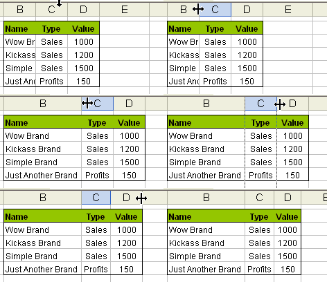 This is my favorite. Select the columns you want to adjust width for. Double click on the column number separator line. The column width is adjusted automatically. This is a very useful way to format your tables. See the screencast aside:
You can use the same technique to adjust row heights.
Select Non-Contiguous Ranges using Ctrl+click
Ctrl+Click to select non-contiguous cells. Useful when you need to format cells matching a particular criteria or paste only few cells.
One click stock quotes with Alt+click
To get stock quotes in excel, enter a company stock symbol in the cell, alt+click on it to launch research pane. (works excel 2003 and above). Find out more.
Move selected cells by dragging the thick black line
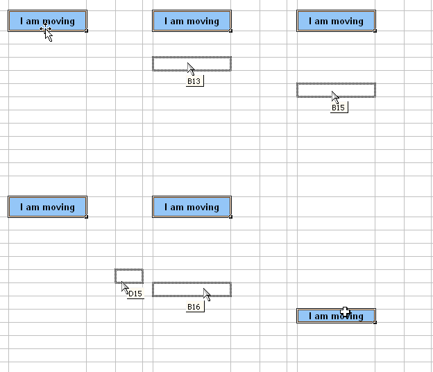
First select a bunch of cells, now drag the thick boundary line to move the cells. Better and faster that ctrl+x, ctrl+v.
Auto fill by dragging cells
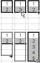
Ok, this is well known, but just in case you don’t know: You can auto fill a range with sequential numbers, dates, days of week, months etc. by entering first few values and then selecting them and dragging the range by clicking & holding the bottom right corner. When you do this excel will automatically fill the rest of cells with data based on what you are entering.
You can also customize excel lists so that you can auto-fill, lets say bank holidays in your country or types of beer in your pub. One more auto fill trick.
What is your favorite mouse based productivity hack?
Share with everyone using comments. Teach me a new trick and show that mice can indeed kick butt.
This is part of our Spreadcheats series, a 30 day online excel training series for office goers and spreadsheet users. Join today.


36 Responses
IMHO, keyboard is also useless when working with the width and height of shapes (buttons, comments, textboxes etc.). I use mouse also when selecting a color of the text or cell interior.
Btw – what keyboard shortcut we use to autofill a range of cells? I used to know it, but I forgot. 🙁
hi, love that weekend autofill trick. And by the way, do you mean “Non-Contiguous Ranges” above? Or maybe i’m being stoopid and missing the joke…
Double-click the bottom right corner to copy down formulas. As well as your first one, column auto width.
Here are a few I use, off the top of my head.
CTRL+scrollwheel to zoom in and out of a worksheet.
Right-click on the worksheet navigation arrows (bottom left) and you can go straight to any worksheet – handy for workbooks with a lot of worksheets, much quicker than scrolling along.
Right-clicking on the statusbar about 1/4 away from the right–hand edge gives you the option to count, sum, average etc. the currently highlighted range.
I also use the mouse to resize/move chart data ranges. If you click on a chart then the data sources are highlighted in different colours. You can then drag and resize the bounding box as you would expect to modify the chart data.
alt+resize with mouse to make charts or other shapes snap to the grid.
I mean right this (http://chandoo.org/img/a/auto-fill-cells.gif) using the keyboard. I’m not sure, but I think there used to be a shortcut to do that. :-$ A regular filling with standard numbers.
Do you mean the Research Pane has value? It’s not just what happens when I click the wrong the button on the right-click menu?
Agree on non-contiguous. Also applying styles with the keyboard is painful. Particularly the comma style with it’s own little toolbar button up there.
Invest in a good mouse that has lots of buttons. Logitech or Microsoft have some good models. I use the software that comes with the mouse to program functions into the buttons. For example, I have configured the two side buttons to move to the next / previous worksheet. I have mouse wheel that can move left or right. I have programed this to pan left or right. Workbook navagation is now so intuitive. My love for excel has vastly impoved with this new functionality. I will never go back to using and ordinary mouse. Look for the Logitech G5, G9 or Revolution MX. A good mouse will be one of the best investments you’ll ever make.
double click the right side of the horizontal scroll bar to split the worksheet vertically from the present cell and top side of the vertical scroll bar to split the worksheet horizontally.
Double click the split line/image to remove the same.
select the worksheet and double click on any column adjust the width of all the columns
@Struzak: Totally agree, when working on drawing shapes etc, mouse beats keyboard hands down. That applies to formatting a bunch of cells (especially colors, fonts etc.)
You can autofill using menu shortcuts – alt+e+i+s (also, ctrl+D can be used, but it doesnt seem to do the series fill)
@artful dodger: duh! my mistake, I am stoopid. corrected it and posted a comment earlier which went missing.
@Leonel: thank you, it is surprising MS has coded so many cool things with double clicks, ctrl+clicks etc but never really documented them (or hid them under heaps of documentation). Finding one of these shortcuts is like winning a prize for your continued use of excel.
@Gordon: “I also use the mouse to resize/move chart data ranges. If you click on a chart then the data sources are highlighted in different colours. You can then drag and resize the bounding box as you would expect to modify the chart data.”
Didnt know this, thanks a lot for sharing this. I am sure I can save few mins using this everytime I work on chart.
@iesmatauw: Thank you… few more tips for you.
holding shift while resizing objects ensures that dimensions are preserved.
holding ctrl will resize keeping the center of the object same (thus resizing on all directions)
when moving objects, charts, holding shift will ensures that either horizontal or vertical position remains same.
when moving objects, charts, holding ctrl will create a copy of the object and places it wherever you move.
@Dick: “Do you mean the Research Pane has value? It’s not just what happens when I click the wrong the button on the right-click menu?” hmm… debatable, but I guess it has few good uses, especially thesaurus, stock / company research. Btw, for comma formats, ctrl+shift+1 works, although I end up using the toolbar buttons more often than pressing 3 keys.
@Alex V: totally agree, my productivity went through roof when I bought the MS wireless optical mouse 200 & keyboard. Although it doesnt have any extra buttons (I find too many buttons on mouse a bit odd) I just like the accuracy of the mouse and its response. Investing in a good kb, mouse, monitor is mandatory if you work long hours in front of computer.
@ketan: “double click the right side of the horizontal scroll bar to split the worksheet vertically” wow, that is a fantastic little trick. thank you for sharing it 🙂
Click on scroll wheel, direction four arrows(L,R,U,D) will pop-up.
Distance of the arrow from the basic point will decide the speed of scrolling the sheet in that direction. Very helpful for to check the long sheets…
Holding the Shift key while moving cells, specially when moving complete rows or columns. This inserts the cells in the new location and deletes the cells in the old location
Hi Gabriela.
I was looking at all these tips to see if someone knew it and there you go. You knew it. When I teach Excel I sometime refer to this tip as one of my favorite secret weapon.
So one again:
Click a column letter or select consecutive columns
Drag the left or right dark border to the desired position
Hold Shift just before releasing the mouse
The column(s) or row(s) will be ‘moved’ in one step. Works with individual cell or range too.
Thanks for mentioning it.
Font colors and cell colors can be changed 2 different ways with keyboard much faster than mouse. First, you can move your fill color and font color and anything else to the left of the file menu by holding alt and then clicking and holding on it an moving over there. Then, when you press the alt button, it highlites the font/cell color. You press the down key to choose the color and your done. This is espically faster if you are changing to one color all the time since you just press alt + enter. The more complex way is with vba. I have a macro that scrolls though my 4 favorite font colors by pressing one shortcut and 4 favorite cell colors with another shortcut. With this I am 10x faster at changing colors than the anyone with a mouse.
Gordon’s chart data range tip also works on formulas. Double-click on a cell containing a formula, then change the formula’s cell references by dragging the highlighted boundry lines of cells the formula references, which are color-coded back to their reference in the formula.
type in Jan, Feb, Mar and Q1 in A1 to D1 highlight all four cells then drag on the cell handle in D1 will give you a series in side a series quarts within months
Create a list in Excel eg CAt, Dog, Rabbit in 3 three cells. Highlight then Choose Tools Options Custom Lists and Import then OK. Now you can type in cat and drag to get Dog and Rabbit. Similar option under Office Button in Excel 2007
Hi Chandoo,
I guess you dont mind using these 🙂
Adjust width of Column to Auto-Fit highlighted cell(s) contents Shortcut
Alt, O, C, A
Adjust height of Row to Auto-Fit highlighted cell(s) contents Shortcut
Alt, O, R, A
And two more to the kitty 🙂
Adjust width of Column Shortcut
Alt, O, C, w
Adjust height of Row Shortcut
Alt, O, R, E
last, and maybe least? — when cropping an image, use Alt with the mouse for more precise control over “closeness” of cropped edge(s).
[keep up the great work & all the feedback —- Pricele$$!!]
When the mouse is over the ribbon the scroll wheel scrolls through the ribbon tabs.
Ctrl and scroll wheel zooms in and out in 15% increments
To insert new cells within a range (and move existing cells in the current column only, down), instead of right click or menu/button Insert – Cells – shift cells down – OK:
Hold down SHIFT and click and drag the Autofill handle (little black box in RH btm corner of selected cell outline) down for the number of cells you want to insert below the selected cell. You will notice the mouse shape changes to a window splitter shape (vertical double-headed arrow with perpendicular double line).
its better to use keyboard to autosize row/column..
ctrl+enter – select column
shift+enter – select row
after either ctrl+o+c+a – autofit column
or ctrl+o+r+a- autofit row
Hello Nitesh,
Are you sure you don’t mean Ctrl+Spacebar and Shift+Spacebar.
Ctrl+Enter keeps the active cell in the same cell after entering a value and Shift+Enter moves the Active cell up after entering a value.
Daniel
Alt+O+H+R – To rename a worksheet
Alt+O+H+H – To Hide a worksheet
Alt+O+H+U – To Unhide a worksheet by selecting the sheet you want to unhide.
Thank you Chandoo for your blog which is really awesome. I am sure that one can become awesome by following your blog.
PASTE SPECIAL VALUES
select data having formula
go-to broad black boundary till pointer appears
right click and drag the box where you want and leave
a menu appears, select copy here values only
……thanks datapig
What a collection of keyboard shortcuts!! As an instructor I brag about knowing a extensive collection of them. Let’s see now which one I haven’t seen here……
Here’s a couple that I didn’t find:
Alt+PgDn (or PgUp)
Same as PgDn (or PgUp) but across the worksheet. Fantastic when you use large set of data. Much better than clicking 5 or 6 time on the horizontal scroll bar!
Oh! Here’s a super hot one:
Ctrl+` (the key between Tab and Esc) It is called Accent Grave.
Displays the formulas in the worksheet.
When this feature is On and the active cell contains a formula all referenced cells are colored coded to match the formula. Press the key again to return to normal view. Fantastic to get acquainted with a workbook you’re not familiar with.
Ok I didn’t see Alt+Enter.
Inserts a hard return (Enter) in a cell. Very useful for long labels.
What else. Ah yes hit F3 to see a list of all the range names in your workbook. If you like Range Names then you should know about this.
What about Alt+= to run AutoSum instantly!
Highlight the cells BELOW a range of numbers (using Shift+arrow key) and hit Alt+= Done!
Last one. Commands placed in the Quick Access Toolbar can be accessed by pressing Alt and a number. Customize your QAT to have you top favorite commands (that do not have a keyboard shortcut) at the left. You will be able to access them using Alt+1 or 2 or 3 ….
Enough for one day.
Dan
Could not do without using F2. It will bring you into a cell at the end of the text or formula.
control [ will take you to precedent cells where data is coming from (including closed excel files). Control] will show you dependants.