
This post is part of Excel Dashboard Week
Background:
In 2008, I received an email from Robert Mundigl, which was the start of a life-long friendship. Robert asked me if he can teach us how to make KPI dashboards using Excel. I gladly said yes because I am always looking for new ways to use Excel.
The original KPI dashboards using Excel article was so popular. They still help around 12,000 people around the globe every month. Many of our regular readers and members have once started their journey on Chandoo.org from these articles.
In this article, we will revisit the dashboard and give it a fresh new spin using Excel 2007.
KPI Dashboard – Reconstructed in Excel 2007
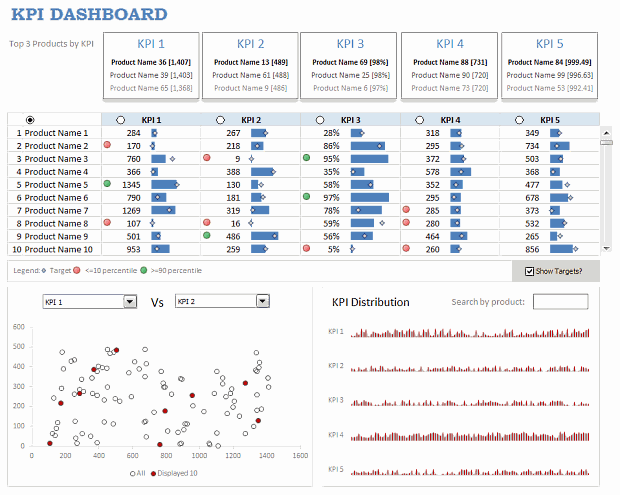
KPI Dashboard – Snapshot
First, take a look at the dashboard I have constructed. This uses almost the same data as Robert’s original dashboard, but adds a lot of new features etc.
KPI Dashboard – Demo Video
How is this KPI Dashboard Constructed?
It would take me 2300 words and 7 cups of coffee to type out the entire instruction. So I will instead tell you what new things I have added to it and how they are done.
Note: For a detailed step-by-step instruction, please consider joining Excel School because this is a 3 part, 120 minute lesson in our class.
Changes to the KPI Dashboard:
I have made the following changes to the original dashboard:
- Added a top bar where we show top 3 products in each KPI
- Added ability to restore to original sort order (as per the input data in Data sheet)
- Instead of showing triangle arrows, used conditional formatting arrow icons – green for values >=90th percentile and red for <= 10th percentile for any given KPI.
- Added individual KPI targets by product (instead of same KPI targets for all products). Also, changed the bar chart visualization to show target markers.
- Added ability to switch on/off the target indicators.
- Added a KPI distribution chart and ability to search by any product.

How are these changes made?
Restoring original sort-order:
For this, I have used the product numbers (values 1 to 100) in Data sheet and sorted them on ascending order. When you click on the product column’s sort button, in the background I just use the product numbers column to sort the KPIs.
Percentile Indicators:
This is the same technique as alert icons in dashboard. Just that I also showed green icons.
Turning on / off the KPI target indicators:
Based on the check-box setting, I return #N/A (thru NA() formula) or actual target value to the chart’s source data range. Rest of the puzzle, you can figure out.
The technique is also explained here: Dynamic Excel Chart with Checkboxes.
Search by Product & Highlight KPI values:
For this I have used an active-x text box and linked it to a cell (L22). Then, I used COUNTIF with wild-card search to locate if a product matches the input or not. [More on the wild-card search technique]
KPI Distribution Chart:
This is an area chart, re-sized to fit inside the space. The red-lines are y-error bars and they are drawn for products that match the search criteria.
Download the KPI Dashboard Workbook
Click here to download the Excel workbook with the KPI Dashboard.
Thanks you Robert:
Special thanks to Robert for such a beautiful dashboard. Visit his clearlyandsimply blog to get some more awesome dashboard / Excel ideas.
How would you have designed the KPI Dashboard?
Share your views on the above dashboard. Also, tell me how you would have designed the same. What charts / tables will you retain. What will you remove and what will you add.
Share your ideas using comments.
More Resources on Excel Dashboards:
- Excel Dashboards – Lots of examples, information and downloads.
- Sales Dashboards – 32 Examples & Download workbooks
- KPI Dashboards using Excel – 6 part tutorial
- Dynamic Dashboards in Excel – 4 part tutorial
- Excel School Dashboard Program – Learn how to make world-class dashboards using Excel


21 Responses
http://bit.ly/hmCink shows a simulation done with http://www.vischeck.com on how part of the dashboard would appear to someone with a common form of color vision deficiency.
oops – I put in the wrong link. It should be http://bit.ly/foZ5Wc .
Chandoo,
many thanks for this post and for revamping the KPI dashboards. I am very happy to hear that the original posts are still so popular.
I love the look and feel of your dashboard and I really like the features you added, especially the sort by product and the Top 3 products section above the KPI columns. Great work. Thanks for sharing.
However, there are some things I would like to put forward for discussion:
1. The individual targets
I like the way you implemented this including the option of checking / unchecking the display. Though, I doubt that there is a real use case where you would define one individual target for a KPI for each product. Usually, if you are comparing a category like products, you will have one common target for all products for each KPI (i.e. 5 targets). In your example you would have to define 500 (!) different targets.
2. The drop downs above the scatter chart
I guess you wanted to make the chart more readable by putting combo boxes above the chart in one line saying “KPI 1 vs KPI 2”. Agreed, it is easier to read. However, I cannot see immediately which one is on which axis. I think this was more intuitive in the original implementation when the drop downs were close to the axes and serving for selection and as an axis title.
3. The area charts / stripe charts
Using an area chart and error bars is a very clever way of implementing this. I also like the “search as you type” functionality. However, I have to say that the charts don’t really tell me much about the distribution of the data. No y-axis, i.e. no context of values. I can’t see the range of all values (i.e. the range between minimum and maximum of all values or of minimum and maximum of the values displayed in the 10 rows of the snapshot), I do not see the average, etc.
Frankly, I would still prefer the box plots to visualize the distribution of the data.
What do you think?
@Naomi… Good point. I should have used the Red to Black series.
@Robert… Thank you so much for your insightful comments.
To be frank, improving your dashboard was a big challenge. You did a very good job of visualizing it. So I went more in experimental direction.
1) I agree that this is not practical. But I want to show a technique so that we can apply similar ideas to other situations. Usually KPIs have standard targets.
2) I agree. I was thinking of adding a label to the chart, somehow missed it. (I mention the same in video too).
3) This is the most experimental idea in the dashboard. I just wanted to see what more can be done. But I totally agree with you. This is the least informative portion of the dashboard.
Dear Chandoo,
Can this kind of dashboards be done on excel 2007????
Regards
Arun
ARUN,
the dashboard Chandoo provides is Excel 2007.
Chandoo… How can a I reduce the numbers of products? I mean, I want only 10 instead 100 products. Thanks in advance
Dear Chandoo,
What does it feel like to be an Excel god?
Cheers.
Chandoo,
How would you go about adding the sort order function into this revision?
@Trois3
Selecting the Option Buttons above the KPI 1-KPI 5 and Product Names Selects the products and sorts them in Descending order by that selection
There is a scroll bar to the Far Right of KPI 5 that allows you to move down to see the other products
.
What else did you want to do?
Dear Chandoo,
dear Robert,
first of all awesome ideas in your KPI dashboard.
Especially the scroll-bar function is very useful!
Now my problem:
I would like to use such a tool via Sharepoint / Excel Services.
Unfortunaltely Excel Services doesn’t support features like form-controls, etc.
Do you have any idea how I could simulate such features with basic Excel features to use such great idea’s (especially the scrollbar) under Excel Services.
Regards Sascha
Dear Chandoo,
dear Robert,
awesome idea’s in the KPI dashboard.
Espeacially the scroll-bar function is very useful.
I would like to use such a function also for a dashboard unter Sharepoint / Excel Services.
Unfortunately Excel Services doen’t support features like form-controls:
Do you have any idea how I could simulate such a funktion like scroll-bar with general excel feature?
Regards Sascha
Chandoo and Robert,
Really great dashboard. I’m going to incorporate this into a project I’m working on right now.
The only thing I can’t figure out is how to incorporate the spinner. What formulas in the calculations tab would I need to modify, and how would I do this?
Hi.
Congratulations. Done everything so far.
My problem is:
1 – My “DATA” sheet doesn’t have a “steady” n.º of items.
2 – I have MORE than “product name”. I have aditional columns. Imagine something like “business unit” (BU=1;2;3;…….)
3 – There is a new chalenge by point 2: How to make the SAME (excelent thing), but being able to FILTER one of those extra fields(BU=1; BU=2; …..), for instance…?
This chalenge has both problems:
First, you must have a way to “link” some kind of “input box” to know the wanted BU
Than you’ll have to get it filtered
Than you will have (in calculation sheet) different count of Item’s (Products).
How can it be done??
It is EXACTLY both your examples, but in “LIVE MODE”…. 🙂
Regards, António
Antonio,
1. As already mentioned in my reply to your other comment you can define named formulas using a combination of OFFSET and COUNT or COUNT A and use those names instead of static ranges.
2. Simply insert the additional columns on the data worksheet, the calculation worksheet and the dashboard and apply the same formulas to those columns as you have in for the product names.
3. Have a look at my reply to John’s comment on the first article of the guest post series. There is a link to a workbook including filter of the dashboard table. Please read also my discussion with John in the comment section to understand the limitations of this approach.
How to implement the target indicators?
Thanks
Hello
your dashboard is amazing,.. all the things you show are really cool, my question is,… do you have a guide about the construction of your dashboard?
you have things I never used in excel like
1. you delete the rows and columns not used, how???
2.how did you create the scroll area?
3.how is that all the sheet is bloqued but your radioButtons and checkbuttons are not.?
4.how did you put actions when your radiobuttons are selected?
well thankyou very much for your dashboard, it really have great ideas.
bye
Chandoo,
Thank you so much for sharing your knowledge to everyone. I plan on taking some of our courses because it’s awesome.
I really like this dashboard. I want to present it to my boss for use in our company. But I had a few questions.
1)How did you reference the Data tab in the Calculations tab where the Original Data table started at the beginning of the table at Data’!B5. When I needed to add more rows to the tblKPIs table (from 100 rows to 1000 rows) I had trouble referencing the first row when I created the array function{=[tblKPIs]} on the Calculations tab. When I tried to recreate the reference it started at row 16!
2)I created a VBA script that I included into the dashboard excel file, and I was able to pull data from my MySQL database. However, I am trying to manage three different sites and create a dashboard for all three sites on different tabs (so, Dashboard tab becomes A Dashboard, B Dashboard, and C Dashboard.)
Now I need to translate the data from MySQL into your tables and tabs, but is there a way to filter the data so that when your calculations tab calculates the information it knows when to exclude data from the data table when it’s not the ‘same’ website.
For instance:
SiteA, Product1, 1, 1000, 0.39, 0.34
SiteA, Product2, 1, 4000, 0.17, 0.34
SiteB, Product1, 1, 6000, 0.44, 0.34
SiteB, Product2, 1, 500, 0.22, 0.34
SiteB, Product3, 1, 5000, 0.43, 0.34
SiteC, Product1, 1, 999, 0.34, 0.34
I am going to create A Data, A Calculations, and A Dashboards, and so on…
What is the best way to filter out the corresponding data into the respective data tables so that it’s clean?
Thanks!
Chandoo, How do I get these to download to my cpu? It pops up as if it is a big cpu formula instead of excel sheets
i think u r being too commercial chandoo…u promote most of ur stuff but u don’t explain the backend of it…Be generous to explain more of your vba codes and complex dashboards…
Hi Chandoo,
Thank you for your help.
I have used a similar layout to the first KPI Dashboard you created.
There only addition I wanted to add from the ones above is the box which shows the ‘Top 3 Products by KPI’.
Could you please show/tell me how I could add this to the report?
Thanks
MVP