
If I need some charting inspiration, I always visit New York Times. Their interactive visualizations are some of the best you can find anywhere. Clear, beautifully crafted and powerful. Long time readers of Chandoo.org knew that I like to learn from visualizations in NY Times & redo them using Excel.
Today let me present you one such chart.
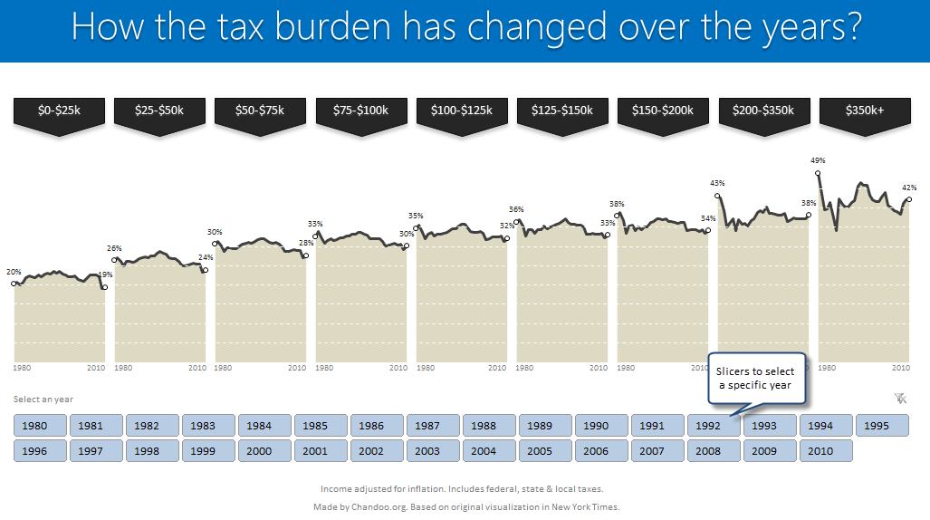
How the tax burden has changed over the years – Visual story by NY Times
First take a look at this story on New York times website. Go ahead and check it out, I will wait for you.
Back already. Good.
Now that you have seen a well presented story with the support of panel charts, let us learn how to re-create such charts using Excel.
Look at the tax burden Excel chart
Take a look at the excel implementation of this chart below. Read on to learn how to create this.
[click here to see larger version]
Recipe for creating this chart using Excel
We need below ingredients to make this chart using Excel
- Raw data
- One area chart and few lines on top
- Simple formulas
- One Slicer (to select an year)
- One large cup of coffee or whatever else that you gulp
So if you are ready, lets start cooking.
Step 0: Arrange data
This is a prerequisite for any charting exercise. Although we can work with data in any shape, for quick results, arrange your data in this format:

In the example file you will find data for overall tax burden for all 9 tax brackets in the years 1980-2010.
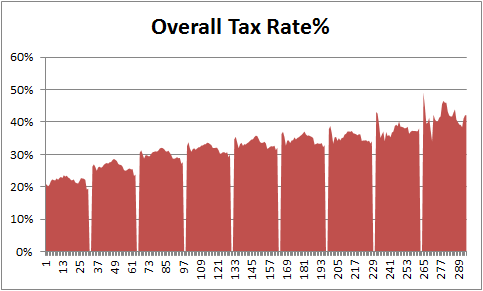
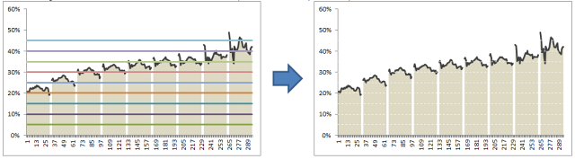
Step 1: Create an area chart from all the data
Simple, select tax bracket & tax percentage rows and create an area chart. This is how it should look.

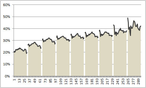
Step 2: Insert 2 columns after every tax bracket in your source data
Very simple, just add 2 blank columns after every tax bracket to your source data. This will change your chart to,
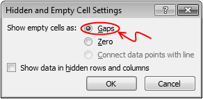
Step 3: Adjust data settings so that blank cells are treated as gaps
Right click on the chart, go to Select Data > Hidden & Empty cells
Specify that all blank cells should be treated as gaps. See below.
Now, your chart should look like this:

Step 4: Add a line to the chart & format it
Although our chart looks almost like NY Times chart, we still need to show a line on top. For this,
- Go to your data, reselect all the tax burden %s and copy them.
- Come back to the chart, select it and paste. (more on this)
- Excel will add this new data as another series to chart
- Right on this new series, choose Change series chart type
- Select Line chart
- Format the chart so that it looks like below.
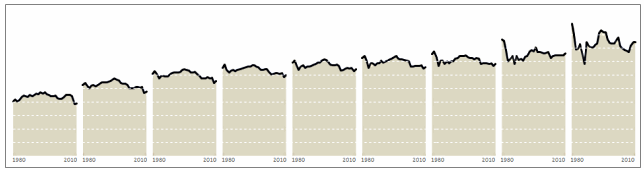
Step 5: Remove grid lines & fake them using additional series
Excel chart’s grid lines always show up behind the data. For our chart, we want them on top. So let just delete grid lines and fake them using additional lines on the chart.
For this,
- In your data, add 9 extra rows at bottom (why 9? because we want to show one grid line for every 5% and the maximum we have is around 45%)
- Fill first row with 0.05, second with 0.1, third with 0.15… ninth with 0.45
- Copy all these and paste them in the chart. You should have nine lines across the chart.
- Now, format each line so that it looks like a dull white line with dashes.
- When you are done, the final output should look like this:
Step 6: Remove horizontal axis (x-axis) labels & fake them too
Again, horizontal axis labels produced by Excel are useless for us. So we will create our own.
- First delete the existing axis.
- Then add a text box to the chart and place it where axis should be.
- Type the values 1980 few spaces 2010.
- Adjust the font size to 7pt.
- Now play with the text box until you are satisfied for one tax bracket.
- Then copy paste it 8 more times and adjust their positions.
Although we could automate this step, it felt un-necessary as the years are not going to change.
Our chart is almost ready
At this stage, our chart looks like below.
It is almost ready, but we need few more additions.
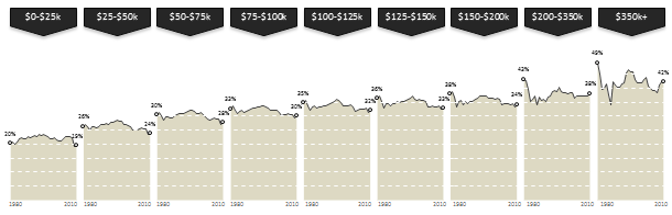
- We need to add labels to first & last point in each tax bracket.
- We need a mechanism so that user can select a particular year.
- When any year is selected, we need to show that year’s tax burden %.
Adding labels for first and last points
This is done by adding one more series of values. This new series (lets call it label-first-last) will have values for only 1980 & 2010. Everything else will be NA().
The formula I used to generate this series is,
=IF(OR(year=1980,year=2010),taxburden,NA())
Once this series is added, we just format it so that only markers are shown (no line) and then add data labels. Format the labels to show in 0% format. Adjust their size and position.
Also add arrow shaped boxes on top to label each tax bracket.
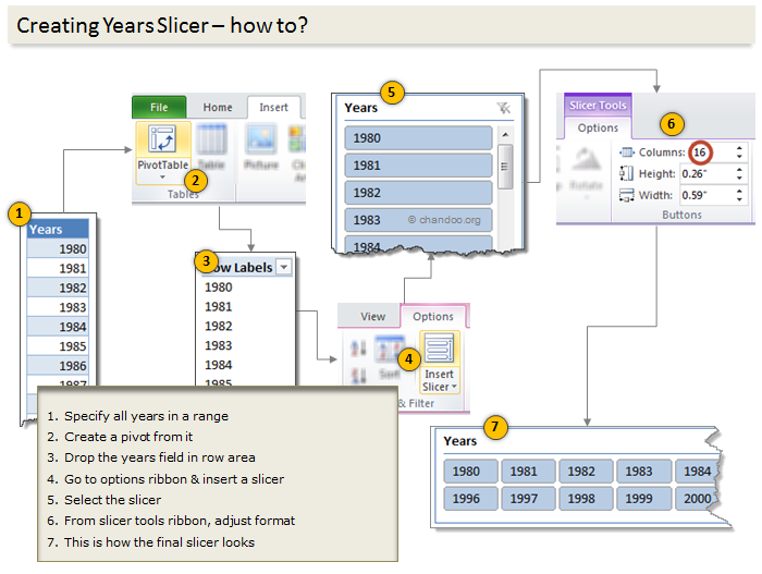
Enabling year selection thru Slicers
[This works only for Excel 2010 or above]
In a blank sheet type the years 1980 thru 2010. Select them and create a pivot.
Once the pivot is ready, insert a slicer for the years field.
For detailed steps on slicer creation see this illustration.
Figuring out which year is selected
Once the slicer is ready, we need to figure out if user made a selection thru slicer. To do this,
- Use a simple formula to check how many values are shown in the pivot table (ex: COUNTA(pivot!A:A) )
- If only one value is shown, then extract it by referring to first row item in pivot (=pivot!A4)
Adding labels for selected year
Once we know which year is selected, we can easily create one more series that has NA() for all values except selected year. The rest you know.
Final outcome – Tax burden over the years chart using Excel
Download this example & Play with it
Click here to download the tax burden chart. Play with it to learn more. Examine the formulas in “Data” sheet & scroll down on “Chart” sheet for step by step instructions.
Do you like this chart?
I really loved how NY Times has been able to tell a very good story by using multiple panel charts. These are great way to examine multidimensional data and understand what is going on.
What about you? Do you like this chart? Please share your thoughts and ideas using comments.
More such charting inspiration
If you are looking for some fresh charting inspiration & ideas, you are at the right place. Check out these examples to get started:
- Introduction to Panel Charts & How to make them in Excel
- Usain Bolt vs. Rest of runners – Interactive visualization in Excel
- Impact of Grammy award on sales – Grammy bump interactive chart
- Visualizing world education rankings – excel chart
- Facebook Privacy policies as a panel chart
- More charts & visualizations
Do you want to create powerful & insightful charts like these?
If you want to learn how to create these types of charts, consider enrolling in our Excel School program. Be warned, you will become unusually awesome in Excel by going thru our course 🙂


26 Responses to “Get busy this weekend, with OR XOR AND [Excel Homework]”
first solution for AND
The two numbers are in A1 and B1
= SUBSTITUTE (SUBSTITUTE (A1+B1*9*9, 9, 1), 8, 0)
regards
Stef@n
next solution for OR
=1*SUBSTITUTE (A1+A2;2;1)
regards
Stef@n
last solution for XOR
=1*SUBSTITUTE (A1+A2;2;0)
regards
Stef@n
Or you could make use of the VBA logical operators!
Define the following as custom functions
Public Function BITXOR(x As Long, y As Long)
BITXOR = x Xor y
End Function
Public Function BITAND(x As Long, y As Long)
BITAND = x And y
End Function
Public Function BITOR(x As Long, y As Long)
BITOR = x Or y
End Function
and then use them such:
A B =BITOR(A,B) =BITAND(A,B) =BITXOR(A,B)
0101 0100 0101 0100 0001
an another solution for AND
=1*SUBSTITUTE (SUBSTITUTE (A1+A2;1;0);2;1)
note:
the binary numbers are in A1 and A2 !
regards
Stef@n
I was obviously playing hooky at the beach during the bit-wise math lesson – you lost me at “Understanding bit-wise operations” 🙂
After looking at the above solutions, I find my solution silly, but still:
For the following formulae,
Row 1: headers,
Row 2: OR
Row 3: AND
Row 4: XOR
Column 1: Input 1
Column 2: Input 2
Column 3: Result
OR
{=SUM(IF(MID(A2,ROW(OFFSET($A$1,0,0,LEN(A2),1)),1)+MID(B2,ROW(OFFSET($A$1,0,0,LEN(B2),1)),1)>0,1,0)*10^(LEN(A2)-ROW(OFFSET($A$1,0,0,LEN(B2),1))))}
AND
{=SUM(IF(MID(A3,ROW(OFFSET($A$1,0,0,LEN(A3),1)),1)+MID(B3,ROW(OFFSET($A$1,0,0,LEN(B3),1)),1)=2,1,0)*10^(LEN(A3)-ROW(OFFSET($A$1,0,0,LEN(B3),1))))}
XOR
{=SUM(IF(MID(A4,ROW(OFFSET($A$1,0,0,LEN(A4),1)),1)+MID(B4,ROW(OFFSET($A$1,0,0,LEN(B4),1)),1)=1,1,0)*10^(LEN(A4)-ROW(OFFSET($A$1,0,0,LEN(B4),1))))}
@Anup
Please don't consider your solution silly
Firstly, You are the 3rd person to submit an answer
Secondly, The best formula/function is the one that you know and understand.
I think I have a very tedious solution, which people won't have the patience to do except in small numbers.
I used the same problem setup as "Anup Agarwal"
AND =IF(AND(MID(B2,1,1)="1",MID(C2,1,1)="1"),1,0)&IF(AND(MID(B2,2,1)="1",MID(C2,2,1)="1"),1,0)&IF(AND(MID(B2,3,1)="1",MID(C2,3,1)="1"),1,0)&IF(AND(MID(B2,4,1)="1",MID(C2,4,1)="1"),1,0)
OR =IF(OR(MID(B3,1,1)="1",MID(C3,1,1)="1"),1,0)&IF(OR(MID(B3,2,1)="1",MID(C3,2,1)="1"),1,0)&IF(OR(MID(B3,3,1)="1",MID(C3,3,1)="1"),1,0)&IF(OR(MID(B3,4,1)="1",MID(C3,4,1)="1"),1,0)
=IF(OR(AND(MID(B4,1,1)="1",MID(C4,1,1)="0"),AND(MID(B4,1,1)="0",MID(C4,1,1)="1")),1,0)&IF(OR(AND(MID(B4,2,1)="1",MID(C4,2,1)="0"),AND(MID(B4,2,1)="0",MID(C4,2,1)="1")),1,0)&IF(OR(AND(MID(B4,3,1)="1",MID(C4,3,1)="0"),AND(MID(B4,3,1)="0",MID(C4,3,1)="1")),1,0)&IF(OR(AND(MID(B4,4,1)="1",MID(C4,4,1)="0"),AND(MID(B4,4,1)="0",MID(C4,4,1)="1")),1,0)
Sorry my last post was totally messed up
AND
=IF(AND(MID(B2,1,1)="1",MID(C2,1,1)="1"),1,0)&IF(AND(MID(B2,2,1)="1",MID(C2,2,1)="1"),1,0)&IF(AND(MID(B2,3,1)="1",MID(C2,3,1)="1"),1,0)&IF(AND(MID(B2,4,1)="1",MID(C2,4,1)="1"),1,0)
OR
=IF(OR(MID(B3,1,1)="1",MID(C3,1,1)="1"),1,0)&IF(OR(MID(B3,2,1)="1",MID(C3,2,1)="1"),1,0)&IF(OR(MID(B3,3,1)="1",MID(C3,3,1)="1"),1,0)&IF(OR(MID(B3,4,1)="1",MID(C3,4,1)="1"),1,0)
XOR
=IF(OR(AND(MID(B4,1,1)="1",MID(C4,1,1)="0"),AND(MID(B4,1,1)="0",MID(C4,1,1)="1")),1,0)&IF(OR(AND(MID(B4,2,1)="1",MID(C4,2,1)="0"),AND(MID(B4,2,1)="0",MID(C4,2,1)="1")),1,0)&IF(OR(AND(MID(B4,3,1)="1",MID(C4,3,1)="0"),AND(MID(B4,3,1)="0",MID(C4,3,1)="1")),1,0)&IF(OR(AND(MID(B4,4,1)="1",MID(C4,4,1)="0"),AND(MID(B4,4,1)="0",MID(C4,4,1)="1")),1,0)
@stefan,
I just couldn't get your solutions to work.
01010101010 + 01010101110 = 02020210120
what am i doing wrong?
@anup
...I got yours to work!
@Stephen - I get the same, but Stef@an's second solution for AND does work (at least for the test cases I used)
@ Stephen / Rich
yes , you are right ! - only this works:
OR
=1*SUBSTITUTE (A1+A2;2;1)
XOR
=1*SUBSTITUTE (A1+A2;2;0)
AND
=1*SUBSTITUTE (SUBSTITUTE (A1+A2;1;0);2;1)
@Stef@n - You're answer is really smart, I never knew about the substitute function before. Great Work!
Thx Michael 🙂
yes - it is simply easy 😉
if you add 1 and 1 - excel calculate 2
and then you have to substitute the 2 - new = 0 respectively 1
Here is a good resource for people wanting to learn binary and hexadecimal.
http://justwebware.com/bitwise/bitwise.html
Three that weren't asked for:
NOT
=SUBSTITUTE(SUBSTITUTE(SUBSTITUTE(A1+A2,0,3),1,0),3,1)
EQV
=SUBSTITUTE(SUBSTITUTE(SUBSTITUTE(SUBSTITUTE(A1+A2,0,3),2,3),1,0),3,1)
IMP
=SUBSTITUTE(SUBSTITUTE(A1+SUBSTITUTE(SUBSTITUTE(SUBSTITUTE(A2,0,3),1,0),3,1),0,1),2,0)
(was using Daniel Ferry's bitwise file to verify against)
@ Kyle
Not only takes one parameter and inverts 0 -1 and 1-0
Took out the +A2
=SUBSTITUTE(SUBSTITUTE(SUBSTITUTE(A1,0,3),1,0),3,1)
Great solutions!
I'll add two:
NAND =1*SUBSTITUTE (A1+A2,2,0)
NOR=1*SUBSTITUTE(SUBSTITUTE (SUBSTITUTE(A1+A2,0,2),1,0),2,1)
This will work for binary numbers of any size (although the text format mask will have to have as many zeroes as there are digits in the longest addend)
Assume binary #s are in C35 & C36, then add and format as text in C37:
=TEXT(C36+C35,"000000000000")
-sum- = 101112211112
AND - SUBSTITUTE 0s for 1s in -sum-, then sub 1s for 2s
=SUBSTITUTE(SUBSTITUTE(C37,"1","0"),"2","1")
OR - sub 1s for 2s in -sum-
=SUBSTITUTE(C37,"2","1")
XOR - sub 0s for 2s in -sum-
=SUBSTITUTE(C37,"2","0")
Just wandered by:
AND:
=SUBSTITUTE(A1+A2,1,0)/2
Clever, Shane. I like that.
[…] post http://www.excelhero.com/blog/2010/01/5-and-3-is-1.html for examples using Sumproduct, and http://chandoo.org/wp/2011/07/29/bitwise-operations-in-excel/ for examples using Text […]
Hi Chandoo,
I am not (yet) really into bitwise calculation, but I am looking for a way to speed up my vba calculation with very big numbers. Would is ben convenient to use bitwise notation for this?
Best regards,
Ronald (the Netherlands)
p.s. love your country!
@Ronald
I'd suggest asking this in the Chandoo.org Forums
https://chandoo.org/forum/
Attach a sample file with an example of some data and describe what you want to achieve