
A while ago, we published a new year resolution template. This was a hit with our readers with thousands of you downloading it. During last week, Peppe, one of our readers from Italy, took this template and made it even more awesome.
The original template had tasks and completion check marks. As you finish each task, you can see overall progress too.
Peppe added priorities to this. With his new version, progress is measured based on how much priority we assigned that particular task. Pretty neat eh?!?
Personal Todo list with Priorities – Demo
First take a look at Peppe’s todo list.

How is this made?
Using lots of Excel goodness of course. The basic components of this todo list are,
- Check boxes – to mark each activity as done (or not done)
- Data validation – to assign priority (1 to 5) to each activity
- Conditional Formatting – to highlight a row when the activity is marked as done
- Thermo-meter chart – to show the progress as you mark each activity done
- Formulas – to calculate % done based on how many activities are done & their priorities.
Since first 4 items are already explained on Chandoo.org, let me focus on the formula part.
Calculating % completion based on priorities:
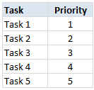
To understand this problem, lets imagine, we have 5 tasks & priorities like below:
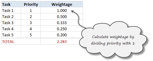
Step 1: Calculating weights
First step is to calculate how much weight each task should get. This is a simple job of inverting priority values (1/priority value). We will get this.
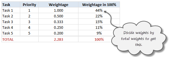
Step 2: Calculate weights to 100%
Next, we adjust the weights so that their total is 100%. To do this, we just divide a task’s weight by total of all task weights.
Step 3: Calculate % done only if a task is marked as done
Now, we just use TRUE / FALSE values generated by the check boxes to calculate % done. For this, we just need to multiply 100% weights with TRUE or FALSE values.
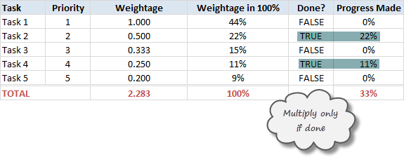
The total of this column gives us how much % of all tasks are done.
Note on weights for priorities
In this approach, we are assuming that doing one priority 1 task gives same output (%done) as doing two priority 2 tasks, three priority 3 tasks etc.
That means the weight enjoyed by priority 1 task is twice that of priority 2 task.
Some other possibilities are,
- Priority 1 is 1, 2 is 0.8, 3 is 0.6…
- A mapping table telling us how much each priority weighs
Read weighted averages in Excel to understand more.
Download this todo list template
Click here to download this template and chase that todo list in style. Examine the formulas in hidden column to understand this better.
Thank you Peppe
I find this template quite simple, yet powerful. It shows how much we can do with Excel by using a little creativity, simple features (conditional formatting, form controls etc.) and a some motivation.
Peppe, Thank you so much for sharing this with us.
If you enjoyed this todo list template, go ahead and say thanks to Peppe.
Also, use comments to share how you handle to dos & pending tasks using Excel. Share your tips & ideas with all of us.
Update
Over in the Chandoo.org Forums, Asshu has updated this witha VB Interface
Have a look and use if from: http://chandoo.org/forum/threads/to-do-list-vb-interface.28973/
More todo lists: Simple todo list in Excel, To do lists & Project Management


144 Responses to “How to add a range of cells in excel – concat()”
You are a god in Excel!
I bow down to you o master of Excel...
You are an absolute legend!
This saved me about 8 hours of 'clicking' not to mention the rsi!!
Thank you, I can't imagine how MS didn't enable this in their concatenate function. What in the world is the point to a function that's less useful than the & symbol.
MS has added this function to Office 2016! It's called TEXTJOIN.
Thank you Chandoo for covering this while MS catches up! (And, of course, users of older versions of Excel still need you on this.)
But... how do I use it?
The formula does not appear when i type in '=conc...' in a cell.
@Hypnos .. thanks alot man 🙂
I think you need to save the downloaded xla file in your excel add-in folder (just select save as and use the excel add-in as the file type, the folder will be shown in the save dialog automatically), let me know if this doesnt work.
Duh!
It didn't work, that is why I wrote... give me some credit dude 🙂 I used to be in your ITCOM.
hmm.. thats tricky, I read that it works that way, it actually did work that way for me, by saving the xla file in the addins folder, i could see and use the formulas. Btw, the formula may not appear when you type =concat... in the cell, but it works nevertheless. Anyways, can you try pasting the code in a module in your sheet and save that sheet as an addin instead... meanwhile I will investigate why this wouldn't work...
that was a great lead to me, and thansk a ton. need you help in this problem. in eh above example if a3 has 'c' but the actual field length should be 8 how do i make use of the same program to create a fixed length text so that i can export it as *.edi file.
In essence i want to create form a excel sheet an exi file withfixed text format having an option to enter headers
@capstri .. thanks for the comments..
let me see if I can help you...
In the above code you can change the for loop to something like this to get the desired effect.
For Each cell In useThis
retVal = retVal + cell.Value + rept(" ",8-len(cell.Value))
Next
you can replace the "8" with whatever fixed lenght you have in mind. Also, I have not tested the above code, you may have to replace the rept() with something else if it throws an error. Let me know so that I will help you if I can... 🙂
[...] Concatenate a bunch of cells using simple formula, Generate tag clouds in excel using vba, Master your IFs and BUTs Tags: Analytics, count, excel, [...]
When I add/save the xla file to my addins directory 'C:\Documents and Settings\colebro\Application Data\Microsoft\AddIns', i double click on the file to install it. When I enter the command =concat(a4:d4) I get the invalid value (#VALUE!). The 'Excel-Udf-Concat' addin is checked iin my add-ins available list. So, I copied your excel code and saved it as an xla file in the add-ins directory, made sure it was 'checked' and still nothing. What am I doing wrong? This add-in will save me a lot of time. - Also, what happens when I send my spreadsheet to another user that does not have your add-in, does the concat still work?
@Colebro: Hey.. that is strange, I remember Amit having similar problem. Did you try copying the code and saving it in to your own excel file in a new module? If you do that, then even if the excel file is sent to another person, the function still works... but if you save it as an add-in then the other computer should also have the addin installed.
Let me know if copying the code helps you... otherwise I will investigate in to this further....
@colebro: Looks like this is not an error with the how you add the add-in but with the add-in it self...
My udf would work fine as long as the input range has strings (text) in them, but when the range has numbers in them the udf would throw #value error. Here is a fix...
replace this part of the code with:
For Each cell In useThis

retVal = retVal + cell.Value + dlm

Next
For Each cell In useThis

retVal = retVal + cstr(cell.Value) + dlm

Next
essentially I am force converting each cell's value to string before creating the concatenated value... this seems to work when you have numbers / dates etc in the cells. Let me know if this helps you...
I must be doing something real stupid because I can not get this to work. I removed the Add-in, changed the statement in the code above and re-added the xla to the add-in. I put a value (either numeric or alpha) and I get an invalid name (#NAME?)
a b c d e
=concat(a1:a6)
#NAME?
BEAUTIFUL - I can't say anything more. THANK YOU SO MUCH! Now, if the function could just skip blank cells...in other words, if in concat(b1:b8,"; ") there were 3 blank cells, it wouldn't return something like this
text 1; text 2; text 3; ; ; text 6; ; text 8
but instead would return only
text 1; text 2; text 3; text 6; text 8
I would fall over and get rugburn on my nose. Even just what you wrote is a huge help - joining large cells, and getting real sick of having to join subsets, then aggregate the subsets in another "overall" concat statement.
🙂 Bring on the coffee dude...this was HELPFUL. So simple, but practical. Now WTH doesn't Excel just make this standard code???????????
LOL - might be too practical for us, right???
@colebro: Oops, I missed to respond to this comment, let me see if I can fix this for you...
Function concat(useThis As Range, Optional delim As String) As String

' this function will concatenate a range of cells and return one string

' useful when you have a rather large range of cells that you need to add up

Dim retVal, dlm As String

retVal = ""

If delim = Null Then

dlm = ""

Else

dlm = delim

End If

For Each cell In useThis

retVal = retVal + cstr(cell.Value) + dlm

Next

If dlm  "" Then

retVal = Left(retVal, Len(retVal) - Len(dlm))

End If

concat = retVal

End Function
this should work... if not try saving the function and your spreadsheet... often excel takes sometime to figure out that the udf is now present. let me know if this doesnt help...
@SheilaC: Welcome to PHD, thanks for the awesome comments... I am happy you found this really useful...
I have added an if condition in the loop to only add the cell if the contents are not blank... hope this helps you in getting that rugburn 😀
Function concat(useThis As Range, Optional delim As String) As String

' this function will concatenate a range of cells and return one string

' useful when you have a rather large range of cells that you need to add up

Dim retVal, dlm As String

retVal = ""

If delim = Null Then

dlm = ""

Else

dlm = delim

End If

For Each cell In useThis

if cstr(cell.value)<>"" and cstr(cell.value)<>" " then

retVal = retVal + cstr(cell.Value) + dlm

end if

Next

If dlm "" Then

retVal = Left(retVal, Len(retVal) - Len(dlm))

End If

concat = retVal

End Function
let me know if this doesnt help...
@SheilaC: you may want to replace the dirty quotes in the code with proper double quotes...
...Sheila would like to reply to Chandoo - unfortunately she is in the hospital with grade 1 rugburn...in fact, they are extracting rug from her nostrils as we speak.
OMG Chandoo - if you were here - I WOULD HUG YOU SO BAD YOU'D SQUEEK! 🙂 Major help like you have no idea. 🙂
Sheila
Other quick edit
change line:
retVal + cstr(cell.Value) + dlm
to:
retVal & cstr(cell.Value) & dlm
Otherwise Excel sends an error when cell.value is a number
@SheilaC : Hope you are alright :P, I am happy this helped you.
@MikeP : thanks for pointing it out, I have changed the code to include your suggestion. 🙂
it was a great help. thanks!!
[...] on text processing using excel: Concat() UDF for adding several cells, Initials from names using excel formulas Categories : Excel Tips | ideas Tagged with: [...]
Very interesting but my dilema is I have a formula in each cell that says VLOOKUP((TEXT(O3,"mm/dd/yy")&A9),Monthly_Data,2) but when the string is not found (which is very likely the majoriity of the time) the result is #VALUE. Can I use an IF statement that says if the string is not in range enter a 0?
@Navneet ... Thanks for the comments 🙂
@EStout ... hmm, I guess you can change the UDF to include a condition to check if the cell has an error then skip it.
here is how:
if iserror(cell.value) = false and cstr(cell.value)“” and cstr(cell.value)” ” then

retVal = retVal & cstr(cell.Value) & dlm

end if
Another way to get this is to modify your vlookup to include some error handling, like
if(iserror(VLOOKUP((TEXT(O3,”mm/dd/yy”)&A9),Monthly_Data,2)),0,VLOOKUP((TEXT(O3,”mm/dd/yy”)&A9),Monthly_Data,2)).If you are using excel 2007 you can try is the iferror function.
Thank you so much!!! It worked.
[...] tip: If you are using formulas to create content in a cell by combining various text values and you want to introduce line breaks at certain points … For eg. you are creating an address [...]
[...] the Concat VBA Function I have written can be used to concatenate a range of cells (along with a custom delimiter), it [...]
The formula that you have shared is for cells that are in a continuous range. How can we edit this for selection of specific set of cells where a filter has been applied ? or the cells that are not in a continuous range?
you have no idea how much time this saved me!!!! thank you so much! i merged 1395 cells into one!
hi chandoo,
a feedback on this UDF in XL2007.
I'm facing problems exactly as colebro's (August 9, 2008).
getting #VALUE! when the range contains numbers (e.g. A, B, 1, D, E)
Is this UDF XL2007-compatible?
ok, please ignore my previous post ...
the codes work when embedded in the target sheet.
if i dump the XLA into Addins folder, it won't work (properly).
also, if the cells have errors (#value!, #div/0!), it gives me "Error 2007"
ok, please ignore the previous post. ..
i got the codes work when embedding it in target sheet.
if i dump the XLA into Addins folder, it won't work (properly)
Also, if the cells contain errors (#value!, #div/0!), concatenated cell shows as "Error 2007"
@Cybpsych: cool... as you can see, the udf is fairly straightforward and simple. I could have made it complicated, but I thought of keeping it simple to handle text concatenation without worrying about all exceptions.
@Morgan: You are welcome. I am happy you found this useful
Help I cannot get the last code to work. I get an error from the following code:
if cstr(cell.value)“” and cstr(cell.value)” ” then
@Daniel: you need to insert = between cstr(cell.value) and "". Same for the next one too. Let me know if you still face a problem. I will try to upload code in a downloadable format.
Ok, I am at my wits end. I have been given a template for my workbooks that I have to use. They include embedded images for headers/footers.
Ex-post-facto development of a complex document, I have to figure out how to incorporate these two images as the left and right headers. However? I use VBA code to generate all my header/footers prior to printing. The workbook has like 40-something sheets.
I can put the image directly into the left header, however it points to a file location for the image on my hard drive. This will cause the logo not to show up when the spreadsheet is downloaded off of the storage location it is placed into. Which is a violation of an official document. rrrrrrrrr!
I tried to link my image to a cell, but there is not a feature to do that in Excel. I can size the image with a row, but it won't show the image when I use code to refer to that cell - however, text in the cell does show up so it is including what Excel sees "in" the cell.
I even tried (grasping here) using a comment with an image background.
Repeat rows does not "see" the picture either.
What can I do????
@SheilaC: which version of excel are you using? In excel 2007, when I have an image in some rows and define those rows to be repeated at top while printing (from ribbon > page layout > print titles) they are properly repeated for each of the pages on the output.
Since you say you are already using VBA to handle some stuff, may be you can think of an out of box solution like transporting excel output to word templates with images already in and then sending them to printers... That is if your version of excel doesnt support images in header rows...
I am using Office 2003. GOD I HATE 2007's ribbons! Why cain't we just keep our dang buttons Mama? Like good little mice we've learned how to push the lever for our pellet, and now - we have to use something that hogs 1/3 of our screen and requires the "Help" function constantly to figure out how to do stuff!!!
NEways, I can't figure it out. It is part of our markings requirements to have these images embedded. So - I'm just leaving off the Left & Right header generation statements in VBA (before print routine), and hard putting them in there using the picture icon in the Header & Footer menu.
But I know, if anyone could've solved this - it's you. You are a VBA GOD!!! 🙂 LOL. My nose is still flat from my last helping here.
PS> How do I open a new thread?
@SheilaC: you said, you have written some VBA to insert images in to the footer. May be you can change code to insert few rows on the top, insert images there and make the rows repeated. That way images need not be copied along with the file.
PS: Unfortunately we dont have any page where you can ask your questions. The usual process is locate the posts that talk about the topic you need help on, just post a comment on the latest post and you should get the response.
Can you please tell me how to add a description to your above UDF like the one that gets displayed in default functions available in excel 2007? Is it also possible to write a help topic on it?
This blog post (along with its precious comments and the replies) contains the most comprehensive coverage of how to concatenate a range in excel (among all the posts I searched on this topic). Thus, I want to further add some nerdy facts to it. Using your above function I created cell references to put in the two default cell merging options in the excel i.e. (a) CONCATENATE function and the (b) using the 'ampersand' sign '&'. The column A had the data to be merged and column B had corresponding cell references of column A i.e. value in cell B1 was 'A1', B2 was 'A2' and likewise. I used the Chandoo's VBA, i.e. =concat(B1:B9,"&"). Using Paste special--->Values and adding an 'equal to' sign i.e. '=' I obtained a formula that would work in excel by default so that there is no need of availability of VBA or the add-in if the file is used on some other systems. Following are some facts that I found,
A formula can have a maximum of 8,192 characters
You can give a maximum of 300 cell references in a single formula using the default "&" (ampersand) sign
You can give a maximum of 30 cell references in a single formula using the default "Concatenate" function (though the function's help states that it can take 255 cell references, my trial didn't go beyond 30)
A single cell can hold a maximum of 32,767 characters. Thus, you can re-Concatenate the above results, which will follow the above conditions regarding cell references, into a single cell till you hit the maximum limit of 32,767.
P. P.S.: I don't know anything about VBA
P.S.: I use MS Excel 2007, you can download my excel worksheet here
P.P.S.: Please do not forget to answer my 2 ques. written at the beginning of this comment 😉
@jUGAD: Welcome to PHD and thanks for such precious comments.
You have found such cool facts about Excel limitations.
Coming to your questions, you can find some material here: http://www.excelforum.com/excel-programming/577764-adding-help-text-to-a-user-defined-function.html and http://www.ozgrid.com/VBA/udf-cat-description.htm
As you can see from the above articles, when you create an UDF you can set description using either VBA or using record macro dialog. I think when you port your UDFs as Add-ins, there will be better control over the dialog etc (not sure though)
Let me know if you learn anything more about this... 🙂
PS: I like your passion and enthusiasm about excel...
Hi Chandoo,
As I had already written in my previous comment that I do not know anything about VBA, further, I had already seen your suggested links before asking from you as I could not find them fruitful even after lots of trials from whatever I understood of them.
It would be great if you could show the complete code here so that I can just copy and paste it 😉
This is AWESOME!! I love this add-in. Works great and saves a ton of work pasting in Word, adding characters, etc.
Thank you for doing this!
@David.. you are welcome 🙂
This is great!! Have you figured out how to comma or semicolon-delimit the resulting string? That would also be really helpful!
@PJ: The function has an option delimiter parameter, you can pass "," or ";" to it and it will delimit the values with that.
Thanks, that worked great! You just saved me a ton of time!
Many, many thanks. Saved me a huge effort too!
Also, if you have a range that has nothing in it, you might find the following useful:
Change
If dlm "" Then
To
If dlm "" And retVal "" Then
That way when there is nothing in the range and you have a delimiter specified you don't get an error when the code tries to subtract the delimiter length from and empty string.
Wade
Great add-in, but it would be even greater if you could add another condition to whas Sheila added. So here goes:
I want to concatenate text in range A1:A100, only if the respective value from range B1:B100 equals to letter "M".
So A1="Sheila", A2="Chandoo", A3="Amer", A4="David", A5="PJ", A6="Ed", A7="Leah", etc.
B1="F", B2="M", B3="M", B4="M", B5="M", B6="M", B7="F", etc.
C1="F", C2="M"
I want D1 to be all values from column A where corresponding value from column B equals whatever is in C1 ("Chandoo, Amer, David, PJ, Ed")
I want D2 to be all values from column B where corresponding value from column B equals to whatever is in C2 ("Sheila", "Leah").
Also, this should work without the list being ordered by any of the columns.
I guess the function should take 3 parameters (rangeToConcatenate, rangeToTestCondition, ValueToTestConditionAgainst)
Hi,
is there a way to expand the solution to Amer's question so that if there is also an "Age" column, it will concatenate only the M's between the ages of 40&49 as an example?
So A1=”Sheila”, A2=”Chandoo”, A3=”Amer”, A4=”David”, A5=”PJ”, A6=”Ed”, A7=”Leah”, etc.
B1=”F”, B2=”M”, B3=”M”, B4=”M”, B5=”M”, B6=”M”, B7=”F”, etc.
C1="41", C2="46", C3="37", C4="59", C5="42", C6="23", C7="35"
D1=”F”, C2=”M”
E1="40", E2="49"
I want F1 to be all values from column A where corresponding value from column B equals to whatever is in C1 and where corresponding value from column C is greater than or equal to E1 and less than or equal to E2 (“Chandoo”, “PJ”).
Is this possible?
@Mairag
Please ask a question at the Chandoo.org Forums and attach a sample file at:
http://chandoo.org/forum/
Thanks Hui,
I have raised a new threade at http://chandoo.org/wp/2008/05/28/how-to-add-a-range-of-cells-in-excel-concat/ and attached a sample file.
ooops, sorry, wrong link
The correct link is http://chandoo.org/forum/threads/concatenate-with-multiple-test-criteria.23172/
@Mairag
and I answered it 5 minutes after you posted it
@Mairag
you can sue the following code
Function ConcatIf(Src As Range, ChkRng1 As Range, myVal1 As String, Optional ChkRng2 As Range, Optional myVal2 As String, Optional Sep As String) As String

Dim c As Range

Dim retVal As String

Dim i As Integer

retVal = ""

i = 1

For Each c In ChkRng1

Debug.Print i; c, myVal1, CStr(ChkRng2(i)), myVal2

  If c = myVal1 And ChkRng2(i) = myVal2 Then

    If WorksheetFunction.IsNumber(Src(i)) Then

      retVal = retVal + Trim(Str(Src(i))) + Sep

    Else

      retVal = retVal + Src(i) + Sep

    End If

  End If

  i = i + 1

Next

ConcatIf = Left(retVal, Len(retVal) - Len(Sep))

End Function
In use it will be
=ConcatIf(Rangge to Concatenate, Rng1, Val1, Rng2, Val2, Separator)
=ConcatIf(A1:A9,B1:B9,"h",C1:C9,"i",", ")
Will concatenate A!:A9 where B1:B9=h and C1:C9=i with a , and a space as a separator
=ConcatIf(A1:A9,B1:B9,"h",,,", ")
Will concatenate A1:A9 where B1:B9=h with a space as a separator
=ConcatIf(A1:A9, B1:B9, "h")
Will concatenate A1:A9, where B1:B9=h with no seperator
@Amer... you can use a simple IF along with helper column so that you show the value only if the testCondition is "M". Then pass the new helper column range to concat.
Of course, you can write another UDF, but such a formula becomes less generic..
Thanks a lot for your formula. It flawlessly concatenated a range of 100 fields yesterday!
- Milco
@Amer
You could also use array formulas rather than helper columns. Just change the range's type to variant so that it will accept an array as input.
My application was to augment the rows of a pivottable (an inventory) with a list of textual codes (identifying the applications for which the item is used) taken from the rows in which the item's name appears in the source table.
So I use:
{=IF(A5"",concat(IF(A5='Lesson Items'!$C$2:$C$250,'Lesson Items'!$A$2:$A$250,"")," "),"")}
where 'Items' is the sheet with the items listed by application, with item names in C and application names in A; and where A5 holds the item name in the current row of the pivottable. I was really frustrated by the lack of 'concatenate' as an aggregation function in pivottables, but this method seems to work pretty well.
For those unfamiliar, remember that you don't actually type the curly brackets "{" and "}"; you type in the formula and hit "ctrl-shift-enter" rather than just "enter", and Excel processes it as an array formula, marking it as such with the brackets.
Here's the version of the function I used:
Function Concat( _
myRange As Variant, _
Optional myDelim As String = "" _
) As String
Dim myRetv As String
For Each v In myRange
If v "" Then
myRetv = myRetv & v & myDelim
End If
Next v
If myRetv "" And myDelim "" Then
myRetv = Left(myRetv, Len(myRetv) - Len(myDelim))
End If
Concat = myRetv
End Function
Sorry about the formatting of my last post. I didn't realize whitespace wouldn't be preserved.
Hey Chandoo/PHD! I just wanted to comment that this helped me out at work a TON! I spread the knowledge and it's helped a few others as well.
One question - is there any way to get the current UDF to IGNORE text values?
EXAMPLE:
=concat(A23:A420,",")
The intent here is to simply grab each number in all of the cells - except in that range, there are text values too. I created merged cells as a sort of "header" breaking up sections of the sheet. So, I'm getting back...
Week1,Task ID,982,989,1010,2221,Week2,Task ID,2213,3222,Week3,
I want to IGNORE any text values and just have it grab the numbers so I get something like:
982,989,1010,2221,2213,3222
Any help is appreciated! AND! I've added your site to my iGoogle. This is awesome 😀
I added another IF/THEN/ELSE statement to avoid placing the last deliminator
Function concat(useThis As Range, Optional delim As String) As String
' this function will concatenate a range of cells and return one string
' useful when you have a rather large range of cells that you need to add up
Dim retVal, dlm As String
retVal = ""
If delim = Null Then
dlm = ""
Else
dlm = delim
End If
For Each cell In useThis
If CStr(cell.Value) "" And CStr(cell.Value) " " Then
If retVal "" Then
retVal = retVal + dlm + CStr(cell.Value)
Else
retVal = CStr(cell.Value)
End If
End If
Next
If dlm = "" Then
retVal = Left(retVal, Len(retVal) - Len(dlm))
End If
concat = retVal
End Function
and here's a modification that will concat only if they contain specified content
Function concatonly(useThis As Range, contains As String, location As Integer, Optional delim As String) As String
' this function will concatenate a range of cells if they contain a search string and return one string with optional deliminator
' useful when you have a rather large range of cells that you need to add up
' format is concatselect(range, search string, search type (0 includes, 1 begins with, 2 end with), Optional deliminator)
Dim retVal, dlm As String
Dim stringfound As Boolean
Dim searchstring As String
If location > 0 Then
If location > 1 Then
searchstring = "*" + contains
Else
searchstring = contains + "*"
End If
Else
searchstring = "*" + contains + "*"
End If
retVal = ""
If delim = Null Then
dlm = ""
Else
dlm = delim
End If
For Each cell In useThis
stringfound = cell.Value Like searchstring
If stringfound = True Then
If CStr(cell.Value) "" And CStr(cell.Value) " " Then
If retVal "" Then
retVal = retVal + dlm + CStr(cell.Value)
Else
retVal = CStr(cell.Value)
End If
End If
End If
Next
If dlm = "" Then
retVal = Left(retVal, Len(retVal) - Len(dlm))
End If
concatonly = retVal
End Function
' By the way: Thanks for posting this code - it's gotta be the best add-in I've seen
This worked perfectly...what a time saver! Thank you so much!
hey mate, thanks for code.... BUT I'm trying to concatenate numbers
eg:
250
260
261
262
402
448
When i use your code it gives me the result: 250251252253254255256257258259260261262263264402448
I don't want the 251 - 259
I should be seeing:
250260261262402448
Please help... I've got about 200 strings to concatenate by tomorrow each of about 120 characters!!
Thanks 🙂
Brad
Try the following code which must be put in a Code Module
To use =Concat(A1:A10)
.
.
Function Concat(useThis As Range) As String
Dim c As Range
Dim retVal, dlm As String
retVal = ""
For Each c In useThis
retVal = retVal + Trim(CStr(c.Value))
Next
concat = retVal
End Function
Here is a function that I have posted in the past (and which Debra Dalgleish is hosting on her site) that others may find useful (you can intermingle cells, ranges and text constants along with an optional delimiter). See this link...
http://www.contextures.com/rickrothsteinexcelvbatext.html#combine
AWESOME!!!! thanks for quick response!!! exactly what i needed
hiho!! really nice code ;D exactly what i needed too
but i'm trying to aggregate something with that function and i can't get it work... i you know a way, I wold be glad
is to add an boolean, if its true it count the number of rows. if it's TRUE it count cells with values and if is more than 1 in the last it remove comma before the value and put " and " before the value. like:
January - March - October - ... - December
with the actual function: January, March, October, December
what i'm looking:January, March, October and December
@Flex
like
=Concat(A1:A10," - ") or =Concat(A1:A10,B1)
Just change the code to the following
.
Function Concat(useThis As Range, Optional sep As String) As String
Dim c As Range
Dim retVal, dlm As String
retVal = “”
For Each c In useThis
retVal = retVal + Trim(CStr(c.Value)) + sep
Next
Concat = Left(retVal, Len(retVal) - Len(sep))
End Function
@Flex
Didn't read your full question
The following should answer all your queries
use as
.
=Concat(A1:A10)
JanFebMarApr...Dec
.
=Concat(A1:A10,", ")
Jan, Feb, Mar, Apr..., Dec
.
=Concat(A1:A10,", ",1)
Jan, Feb, Mar, Apr...Nov and Dec
.
===
Function Concat(useThis As Range, Optional sep As String, Optional last As Integer) As String
'
Dim c As Range
Dim retVal, dlm As String
Dim NE As Integer, NC As Integer
Dim i As Integer
'
retVal = “”
'
NR = useThis.Rows.Count
NC = useThis.Columns.Count
noitems = Application.WorksheetFunction.Max(NR, NC)
'
If last = 1 Then noitems = noitems - 1
For i = 1 To noitems
retVal = retVal + Trim(CStr(useThis(i))) + sep
Next
If last = 1 Then retVal = Left(retVal, Len(retVal) - Len(sep)) + " and " + useThis(noitems + 1) + sep
'
Concat = Left(retVal, Len(retVal) - Len(sep))
End Function
answered really fast ;o
oh, i was even close..! but MANY. THANKS the result was exact what was expecting to be.
thanks for the code, will be really useful.
hmm, here again!
i found something.. when the last cell in the range is blank ("") the function don't put the " and ".
And if the last cell in the range it's a number, it returns #error.
i have to stop here for today, but i changed the code using lines of the function on the top of the page, to ignore the blank cell in the range(not working properly if blank cell is the last).
here is:
Function Concat(UseThis As range, Optional sep As String, Optional last As Integer) As String
Dim c As range
Dim retVal, dlm As String
Dim NE As Integer, NC As Integer
Dim i As Integer
retVal = ""
NR = UseThis.Rows.Count
NC = UseThis.Columns.Count
noitems = Application.WorksheetFunction.Max(NR, NC)
If last = 1 Then noitems = noitems - 1
For i = 1 To noitems
If CStr(UseThis(i).Value) "" And CStr(UseThis(i).Value) " " Then
retVal = retVal + Trim(CStr(UseThis(i))) + sep
End If
Next
If last = 1 Then
If CStr(UseThis(i).Value) "" And CStr(UseThis(i).Value) " " Then
retVal = Left(retVal, Len(retVal) - Len(sep)) + " and " + UseThis(noitems + 1) + sep
End If
End If
Concat = Left(retVal, Len(retVal) - Len(sep))
End Function
'''''''''''''''''''''''''''
@Flex
People always find a case you don't test for
Try this
===
Function Concat(useThis As Range, Optional sep As String, Optional last As Integer) As String
Dim c As Range
Dim retVal, dlm As String
Dim NE As Integer, NC As Integer
Dim i As Integer
Dim noItems As Integer
retVal = ""
NR = useThis.Rows.Count
NC = useThis.Columns.Count
noItems = Application.WorksheetFunction.Max(NR, NC)
If last = 1 Then noItems = noItems - 1
For i = 1 To noItems
retVal = retVal + Trim(CStr(useThis(i))) + sep
Next
If last = 1 Then retVal = Left(retVal, Len(retVal) - Len(sep)) + " and " + Format(useThis(noItems + 1), "General Number") + sep
If last = 1 And useThis(noItems + 1) = "" Then retVal = Left(retVal, Len(retVal) - Len(sep) - 2)
Concat = Left(retVal, Len(retVal) - Len(sep))
End Function
Hi,
I have tried various options offered, but have not seen a fit for my challenge.
I have a large range of values in a column. ie B1="Hello" B2="There" b3= "How?" etc. I would like to concat them based on a value in another column. For example A1=1, B1=1, c1=1. Basically I want to use a formula to define my range as I have additional values I want to concat seperatly in lower cell ranges. ie b4="good" b5="Bye" A4=2, A5=2. Any suggestions?
Thanks a million!
@Mike
If I understand you correct you want to have a Concat If function
That is concatenate values if other values meet a criteria
.
I have written a small UDF below which will do just that
.
Use
=Concatif(Concat Range, Validation Range, Validation, [Seperator])
Concat Range is a range of Values/text you want to concatenate together
Validation Range is a range of Values/Text you want to comapre to a Validation value
Validation is a Text or Number you want to compare the Validation range against
Seperator is an Optional seperator and is a Null if not supplied
.
eg:
=concatif(B1:B5,A1:A5,1)
Will concatenate the Values in B1:B5 where A1:A5 = 1, with no seperator
=concatif(B1:B5,A1:A5,"Tom","-")
Will concatenate the Values in Columns B1:B5 where A1:A5 = "Tom", with a - seperator
=concatif(C12:G12,C14:G14,"John","-")
Will concatenate the Values in Rows B1:B5 where A1:A5 = "John", with a - seperator
=concatif(C12:G12,A1:A5,D1,"-")
Will concatenate the Values in Rows B1:B5 where Column A1:A5 = Cell D1, with a - seperator
.
You may need to check the " and - characters in VBA
Hui,
I greatly appreciate the help. You have no idea!
I tried the function, your 4th example is the one I am attempting to use.
Unfortunatly I am getting a compile Syntax error. On what looks like the last line :ConcatIf = Left(retVal, Len(retVal) – Len(Sep))
I tried it on a simple mock up
in cell D1= concatif(B1:B4,A1:a4,C1,"-")
Column A Column B column C
123 X 123
123 Y
456 Z
456 Q
Any other thoughts
Yes
Your formula is ok
Note my very last line after the code
.
Retype the - sign on the line
ConcatIf = Left(retVal, Len(retVal) – Len(Sep))
even though it looks like a - it probably isn't
.
In VBA if a line is highlighted Red there is something wrong with the syntax
Awesome! Awesome! Awesome! I bow down to you Sir. Thank you.
Thank you so much! I kept getting a #VALUE! error, when there was too much text (only like 200 characters... excel 2010), when I would delete certain parts, like parentheses out of the text it would work, however due to the nature of the text, I needed them. Anyways, this code did the trick, also I got the range code added it, sure saved a long list of cells!!!
This works perfectly for letters, but when I try to use numbers, I get a #VALUE! error. Any ideas? Using excel 2010.
@Wouter
Try the following which has been slightly modified
Wonderful code. I have just started using excel 2010 and use the code to create a string that the "get external data - msn stock quote function" works from. With msn now no longer supporting the stock quote addin (excel 2003) I was using, I found this code a god send. I have large list of stocks and this code has saved me from doing a massive concatenate formula. Brilliant, love it, thank you.
More than 3 years after the original post and this is still helping people! I took the version you (Chandoo) wrote for Sheila and then added the bit that Jive contributed to leave out the last delimiter (at the end) and it is absolutely perfect and saved me from what would definitely have been a major migraine. THANK YOU!!! FYI, I used this in MS Excel 2010.
This is a great function and I'm impressed with the discussion too.
I did not find in the comments way to concatenate numeric cells as strings.
I have custom format in Excel (“Text”0000, which gives me numbering Text0001, Text0002, etc) that actually stores numbers in cells. The concat UDF returned 1, 2, 3, ... as a result instead of Text0001, Text0002, Text0003, ...
Well, I googled another solution, instead of using cell.value I used cell.text, it worked.
So, these lines
[code]For Each cell In useThis
if cstr(cell.value)"" and cstr(cell.value)" " then
retVal = retVal & cstr(cell.Value) & dlm
end if [/code]
I changed to these
[code]For Each cell In useThis
if cstr(cell.text)"" and cstr(cell.text)" " then
retVal = retVal & cstr(cell.text) & dlm
end if [/code]
Cheers
Mihajlo
Well done & Correct
As you've discovered
cell.Value returns the Value
cell.Text returns the displayed Text
This is great where you want date strings
Thanks for this.
I had a need to concatenate a range, quickly discovered the limitations of the built-in function, quick Google search, found your solution, pasted the code into the VB editor and voila.
You've saved me hours of head scratching and frustrations.
Thanks! This worked for me and it was exactly what I needed to use in Excel 2010.
Thank you! You're doing the lord's work!
Hey there! This is a great function and has proved to be very useful, but I've run into what seems to be the same problem that Alex posted on May 2nd. I'm using concat() to dynamically concatenate a range of cells (because I didn't know about the ConcatIf() function before finding it in these comments, but the work is basically done and I don't feel like changing it if I don't have to :P) and once I get over 100 cells that meet my criteria I get a #VALUE error. I need it to concatenate up to ~180 cells at most, so at the moment I can't use this function almost half of the time. HALP! Thanks again!
@Joe
.
There should be no limit (until you run out of memory) to the number of cells you can Contaif
.
I am able to easily Concatif 500 cells of 10 characters together using the Code from Post No. 70.
=Concatif(A1:A500:B1:B500,1)
.
Can you be more specific about what your doing or send me your file?
This is awesome. Thank you so much for creating it. You saved me soooooo much time.
This was so IMMENSELY useful. Thank you so very much for posting this Chandoo!!!
When using this add in, I'm trying to use it on at least 15 cells, but it gives me a value error. If I reduce it to 5 cells, it will work. Any thoughts?
Thanks for the CONCAT() plug in, very helpful! I've concatenated a HUGE range (over 400 cells) and the result is almost 12,000 characters. Excel tends to truncate the _display_ of all characters however. I'm convinced the formula works as advertised because if I copy the cell into Word or Notepad, all the characters are there. This is not a complaint! 🙂 Just an fyi for anyone who might experience the same behavior.
Thanks. Dave
Thank you guys for such a great code, I found the concatif very helpful, but would you please help me with my case?
I have the following list to concate
# Code Value
1 22 1001
2 22 1002
(Blank) (Blank)
3 22 1003
4 22 1004
5 22 1005
(Blank) (Blank)
7 22 1006
.
.
so on
How can I concate Value with Code=22 and start from #3 to the last of the list?
ConcatIf(Value, Code, 22, ", ", StartFrom (#3))
Wonderful, just what I needed! Thanks for sharing!
This really helped! Thanks! I had a column of data (numbers wrapped in quotes and suffixed with a comma) and this enabled me to place them all in one cell, one one line so I could then export this list into a WQL/SQL query. Saved a lot of time. Thanks again.
Just found this great function from a google search. It Rocks!! It works easily and will especially help me when I do concatenated text data sends back into our FP&A system.
I also love that it can give me just the results of cells that are full when I check very long ranges with blanks in it. Plus it is fast too.
Thanks so much. You Rock!! This site has given me so much over the years. Keep up the great work.
[...] Maybe: How to add a range of cells in excel – concat() | Chandoo.org - Learn Microsoft Excel Online [...]
I want to do this without VBA, is it possible ?? when i use the concatenate() func and input a cell range in a column it give a #Value error. however when i manually input cells seperated my comma it is working fine. help me out please.
Thanks
Sushant
@Sushant
Do you want to Concat or Concatif without VBA?
You have limited flexibility to Concatenate ranges without VBA
Can you post a sample file for us to review?
Refer: http://chandoo.org/forums/topic/posting-a-sample-workbook
Use the ADDRESS function nested within the SUBSTITUTE function to get the addresses for the cells you wish to concat (e.g. A5 B5 C5 D5 ... BB5 BC5). Type =A5:BC5, replace braces {} with () and "," with , and type CONCATENATE in front of the left parenthesis. Oh, and delete any remaining " inside the parentheses.
I'm sorry, it should have read:
Type =A5:BC5--press F9--, replace braces {} ...
had I read down the comments first I would have seen that @Hui had already written a concatif() function, however I did not do that before creating my own using the original concat() as inspiration, so here's my own version I hope you find useful
Public Function CONCATIF(criteria As Variant, criteria_range As range, Optional concat_range As range, Optional delim As String) As String
'this function will concatenate a range of cells that meet the specified criteria and return one string
'credit to chandoo.org for the original concat() function extended here to accept criteria evaluaition
'How to add a range of cells in excel – concat() - http://chandoo.org/wp/2008/05/28/how-to-add-a-range-of-cells-in-excel-concat/
Dim retVal, dlm As String
Dim i As Integer
retVal = ""
If delim = Null Then
dlm = ""
Else
dlm = delim
End If
If concat_range Is Nothing Then
Set concat_range = criteria_range
End If
i = 1
For Each cell In concat_range
If criteria_range.Rows(i).Value = criteria Then
If CStr(cell.Value) "" And CStr(cell.Value) " " Then
retVal = retVal & CStr(cell.Value) & dlm
End If
End If
i = i + 1
Next
If dlm "" Then
retVal = Left(retVal, Len(retVal) - Len(dlm))
End If
CONCATIF = retVal
End Function
Regards,
Jim
Name Coins
Ken Douglas 500
Ken Douglas 400
Maria Jones 111
Warren Mayfield 245
Maria Jones 344
Hi,
please look into the above data, I need a favor if anyone plz let me know how should I look coins value in an other column name wise. If I use vlookup It shows me only first value (500) for Ken Douglas.
hi,
can you please help me to concatenate 2 strings in which one string is italics and i want the same format after concatenation. Is this possible?
If you add Chr(10) you can keep page breaks (alt+enter). So the text keep formatting.
Sub FormMergeCells()
Dim result As String
For Each cell In Selection.Cells
If Not cell.Value = vbNullString Then
result = result & Chr(10) & Trim(cell.Value) & ””
End If
Next
Application.CutCopyMode = False
With Selection
.Clear
.HorizontalAlignment = xlLeft
.VerticalAlignment = xlTop
.WrapText = True
.MergeCells = True
End With
Selection.Cells(1, 1).Value = result
End Sub
thank u !!
Concat is great. I was wondering, however, how one could suppress extra separators when a cell is empty. I keep ending up with results like: "Jim,,, Sally, Debbie, Carl,,,,,," when there are empty cells within the range.
@Bob
Chandoo's original code does exactly that, suppresses the blank cells
Which version from above are you using?
Hui...
I used the link to the installer "xla" file. I don't know which version that is. I could copy the original code but I didn't understand where to put it.
@Bob
I think Chandoo updated the code just below the Addin but didn't upgrade the addin.
I have now updated the addin and so the functionality should be as you require.
Hui...
Thanks worked great.
Thanks! you've just saved me so much aggro.
Note to self - time to pick up some vba skills.
Thanks chandoo... saved lot of time
you sir are a genius and a gentleman 🙂
Thanks a ton!
Thanks so much mate!
Hello, I have a little comment about the following line :
Dim retVal, dlm As String
What actually happens here is retVal is declared as a variant type variable, and dlm is declared as a string variable. It is the same as writing this :
Dim retVal As Variant, dlm As String
Try running the code and setting a break point on the next line, you will see this in the immediate window.
What you should use is something like this :
Dim retVal As String, dlm As String
or even better, for better understanding and readability :
Dim retVal As String
Dim dlm As String
@Eric
Although you are correct, there is also nothing wrong with using default values where appropriate
Personally I don't like mixing variable types on one line and so i will keep all my variants on one dim line and strings on another line
I came across your solution as I was trying to code a solution of my own. However, I had a unique complication: I needed to accept an Array as an input instead of Range. Why? Because the inputted Array was being calculated using If statements on arrays of cells. For example:
=IF(Table1[Status]="OK",Table1[ID])
If you press control+shift+enter when entering this formula, Excel returns the array of all values in the column field of Table1 where that row has a status of "OK". Combining this with the concept you introduced above, you could generate a comma-separated list of all IDs where the row is OK.
Because I had started writing my script before I found yours, I used different variable names and slightly different methods. But you can use my technique to extend your script if you wish in order to support either arrays or ranges of cells as an input:
Function ConcatList(ValueRange As Variant, Optional Delimiter As String) As String
On Error Resume Next
Dim xCell As Range
Dim ConcatValue As String
Dim xVal As Variant
If Delimiter = Null Then
Delimiter = ""
End If
Debug.Print VarType(ValueRange)
If VarType(ValueRange) = 8204 Then
For Each xVal In ValueRange
If xVal False Then
ConcatValue = ConcatValue & Delimiter & CStr(xVal)
End If
Next xVal
Else
For Each xCell In ValueRange
If LenB(xCell.Value) 0 Then
ConcatValue = ConcatValue & Delimiter & CStr(xCell.Value)
End If
Next xCell
End If
ConcatValue = Right(ConcatValue, Len(ConcatValue) - Len(Delimiter))
ConcatList = ConcatValue
End Function
[…] you can follow this link: http://chandoo.org/wp/2008/05/28/how-to-add-a-range-of-cells-in-excel-concat/ (one of the best site to learn […]
I love your concat command - that really helped me out. Thanks!
(Re-post to correct email for notification.)
I have been using this great UDF for a while now.
Seems that I always need to sort the values before concatenating them with CONCAT().
Could the function be altered to have an optional argument to sort?
While you are at it, another optional argument for length of cell would be nice. Negative value would take from right, positive value would take from left.
I am able to use this seamlessly by installing this UDF i.e (Just download the concat() UDF excel add-in and double click on it to install it). But i need to share the tool i am building with others and since i have used this formula in my tool, it will not work on others' computer i suppose. Is there a way i can embedd this in my excel file it self so that even if i pass my file to someone else, they can continue to use to file without installing the UDF on their end? Thanks
I have to leave a comment - thank you so much for your code, you have no idea how much time you have saved for me... Thank you again!
Hi Chandoo,
First let me say that your function has saved me countless hours.
Thank you for that.
I just have one tiny issue that I have been trying to get around with no luck.
Your function works perfectly for what I need, but it is also returning duplicate values. Is there a way to edit the function so it doesn't return duplicate values?
Example:
A1 = 100
A2 = 100, 200, 300
A3 = 200, 400
A4 = 200
A5 = 400
Using your function in A6 = 100, 100, 200, 300, 200, 400, 200, 400
Is there a way to edit the function only unique values are displayed?
Which would make A6 = 100, 200, 300, 400
Any help would be appreciated.
Here is the version of the function I am using:
Function ConCat(useThis As Range, Optional delim As String) As String
' This function will concatenate a range of cells and return one string
' Useful when you have a rather large range of cells that you need to add up
Dim retVal, dlm As String
retVal = ""
If delim = Null Then
dlm = ""
Else
dlm = delim
End If
For Each cell In useThis
If CStr(cell.Value) "" And CStr(cell.Value) " " Then
retVal = retVal & CStr(cell.Value) & dlm
End If
Next
If dlm "" Then
retVal = Left(retVal, Len(retVal) - Len(dlm))
End If
ConCat = retVal
End Function
This formula is great. Is there a way to make it FILTER smart? I have a long list that needs concatenating, but only after it is filtered by one of several criteria.
When I apply the filter to show only one category, then use the =concat(B2:B43) formula at the bottom of the filtered list, the results include all rows between B2 & B43, not just the rows that match the filter.
Any help would be appreciated.
The simplest way to do this is to use the TEXTJOIN formula.
=TEXTJOIN("delimiter",boolean remove null cells, RANGE)
Is TEXTJOIN is a built-in Excel function? Unbeknownst to you, you have been provided with your own custom User Defined Function that someone called TEXTJOIN. If you looked at the code in TEXTJOIN you'd likely see something very similar to CONCAT.
TEXTJOIN is a built in feature for Exvel2016. It was released in February. If you use older versions of Excel you still have to use the UDF or other solutions here.
That's great that Excel now has that "concatenate a range" function built in, but I still find Excel versions back to 2012 to be very common. Companies are now being slow to upgrade. I won't be holding my breath on that brand new function.
Sorry, I can't get this to work in Excel 2010 32-bit.
I have successfully created the .xlam add-in (xla didn't work), it "finds" the formula, however it never works it comes up with "compile error variable not defined" error message, highlighting "cell" in "For Each cell In useThis"
Please help, thanks
Lyndon
_________________________________________________________
Function concat(useThis As Range, Optional delim As String) As String
' this function will concatenate a range of cells and return one string
' useful when you have a rather large range of cells that you need to add up
Dim retVal, dlm As String
retVal = ""
If delim = Null Then
dlm = ""
Else
dlm = delim
End If
For Each cell In useThis
If CStr(cell.Value) "" And CStr(cell.Value) " " Then
retVal = retVal & CStr(cell.Value) & dlm
End If
Next
If dlm "" Then
retVal = Left(retVal, Len(retVal) - Len(dlm))
End If
concat = retVal
End Function
Hello, I seem to have trouble having this function reference a range to concatenate in a different cell. For example, I have a value in A1 that is the reference for the range I'd like to concatenate (i.e. Sheet1!C1:Sheet1C300). If I were to write the function in B1 as "=ConCat(CELL("contents",A1)," ")", I receive a value error. When I step into the function, it looks like it returns the A1 value as within quotes, which returns a value error for the ConCat function. Is there a way to rectify this?
If I have a list like this
03005021
03005022
03005042
03006023
03006024
03006025
and run the =concat(A1:A6,"|")
I get
3005021|3005022|3005042|3006023|3006024|3006025
The leading zero is dropped. I must havr this leading digit whether it is zero or not.
I have tried everything I can think of.
Is there a way to concat a list without excel doing this truncating?
@TMBadmin: Welcome to Chandoo.org and thanks for your comment.
Replace cell.value with cell.text in the code to get leading zeros.
Years after you write it - you're STILL a legend!!
Thank you soooooooooooo much
I want to concatenate column A and column B cells value with separator using vba. My result will be shown on cell D2
Hi, this is an awesome bit of code, is there any way to insert a line break between each value?
Thanks
@Kelvin
If you continue to read the Comments below the post there are several examples of alternative Concat and Concatif versions of the code
You can always add a Line Feed using char(10)
Hi guys,
just came across this and wanted to add that Excel now has a was easier way of doing this with the TextJoin function. I'm sure you're aware of that already, but thought it might be helpful to others that read this thread.
Cheers
Nadine