VLOOKUP may not make you tall, rich and famous, but learning it can certainly give you wings. It makes you to connect two different tabular lists and saves a ton of time. In my opinion understanding VLOOKUP, INDEX and MATCH worksheet formulas can transform you from normal excel user to a data processing beast.
Today, lets understand how to use these formulas better.
What is the syntax for Match, Vlookup and INDEX?
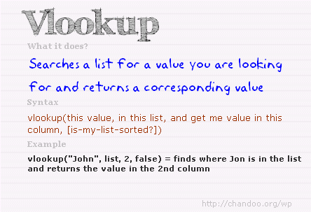
Here is the syntax for these three very powerful functions in plain English:

What are vlookup () and match () ?
VLOOKUP and MATCH are your way of asking excel to find a needle in haystack. Imagine you have all your customer contact information in one sheet in the range A1:D5000 in the format phone number, name, city and date of birth. Now you need to find out which customer has the phone number “936-174-5910”. How do you do it?
You guessed it right, you use VLOOKUP and summon excel to do the search and return with customer name.
While VLOOKUP is used to fetch value a based on what you are looking for, MATCH is used to fetch the position of the value you are looking for.
See this illustration to understand :

What does VLOOKUP really do?
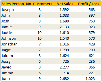
Imagine you have a list of data like this:

Now, how do you answer the question – “How many sales did Jimmy make?“
Yes, your guess is right. VLOOKUP is one of the formulas you can use to answer questions like this.
VLOOKUP searches a list for a value in left most column and returns corresponding value from adjacent columns.
So, in our case, we need VLOOKUP to search for Jimmy and return the amount of sales he made from column 3.
VLOOKUP Syntax & Examples:
The syntax of VLOOKUP is simple:
=VLOOKUP( this value, your data table, column number, optional is your table sorted?)
Here is an example to get you started:

Learn more about VLOOKUP Formula with examples
Please check out this page for 10+ examples of VLOOKUP and how to use it to solve real world problems.
VLOOKUP Examples & Homework
I have made a small excel file detailing 4 VLOOKUP formula examples. The file also contains some home work so that you can practice this formula.
Download VLOOKUP Example Workbook
[NEW] XLOOKUP replaces VLOOKUP in Excel 365
If you are using Excel 365, you can use the new & improved XLOOKUP function. It offers a shorter & more versatile syntax for performing lookups.
For ex: the same lookup as above will be done with XLOOKUP like below:
=XLOOKUP(“Jimmy”, A2:A14, C2:C14) will lookup “Jimmy” in column A and return sales amount from Column C.
Click here to learn more about XLOOKUP.
So what is INDEX() then?
INDEX function is your way of telling excel to fetch a value from large range of values. Since MATCH() function can tell us where the data is found, you can then use INDEX() function to extract corresponding data from another column. In this case, we can use MATCH() to find out which row has net sales 1,799 and INDEX() to return the name of the person. Like this:
Find the position of 1,799 in sales: =MATCH(1799, $C$2:$C$14, 0)
The answer will be 8.
To find the 8th person in names list, we can use INDEX() function like this:
=INDEX($A$2:$A$14, 8)
The answer will be Jagjit.
Related: Learn more about INDEX Formula.
So how are INDEX() and MATCH() linked to each other?
Since MATCH returns the position of the item you are looking for in a list, you can then use this position in INDEX to fetch values surrounding the searched value.
So, we can combine both functions like this:
=INDEX($A$2:$A$14, MATCH(1799, $C$2:$C$14, 0))
This combination is called as INDEX+MATCH formulas.
Related: Using INDEX + MATCH functions & INDEX+MATCH Video
Finally
Remember, both VLOOKUP and MATCH throw a fail error of #N/A if the value you are looking for is not there. If you want to stop seeing the error, use IFERROR function.
Just use them with some dummy data, play around with arguments and see how you can say “oh yeah, I can do that in few minutes” to your boss next time.
VLOOKUP tutorial – video
Please watch this quick video tutorial to understand all these concepts and how to write VLOOKUP formulas easily.
INDEX MATCH Tutorial – Video
Want to Learn More Formulas? Get my VLOOKUP book
If you want to learn VLOOKUP and other Excel lookup functions, then consider getting my VLOOKUP book.


5 Responses to “Preparing Profit / Loss Pivot Reports [Part 2 of 6]”
[...] Preparing Pivot Table P&L using Data sheet [...]
[...] Preparing Pivot Table P&L using Data sheet [...]
[...] Preparing Pivot Table P&L using Data sheet [...]
I am not getting sound from the videos. I have checked all the settings and spent several hours searching the Internet to no avail.
Has anyone else had this problem?
Is there anyway to get the Grand Total to be broken out in the same fashion as the items above it? For instance, if you have in column 1, widget a, widget b, and have their sales by month in column 2, I'd like to see the grand total also be by month, for widget a & b combined.
I can't get anything other than a single line for the grand total, rather than the same format as the data above.
Widget A Month Sales
Jan 100
Feb 200
Widget B
Jan 150
Feb 250
Grand total - here I would also like to have Jan, Feb.
Jan 250
Feb 450