
Excel SUMIFS function is used to calculate the sum of values that meet any criteria. For example, you can calculate the total sales in east zone for product Pod Gun using SUMIFS formula.
In this article, you will learn:
- What is SUMIFS function and how to use it?
- Syntax for SUMIFS
- Using SUMIFS() with tables and structural references
- SUMIFS examples – simple, wild card
- Using SUMIFS() with date & time values
- Free sample file for SUMIFS formula
- More formulas for data analysis
How to write Excel SUMIFS Function?
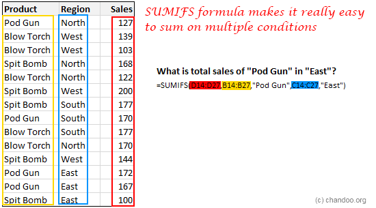
Using SUMIFS you can find the sum of values in your data that meet multiple conditions.
So, to get the sum of all the Blow Torches sold in North, we just write,
=SUMIFS(D3:D16, B3:B16,"Blow Torch",C3:C16,"North")
Similarly to find the podgun sales in East, just write,
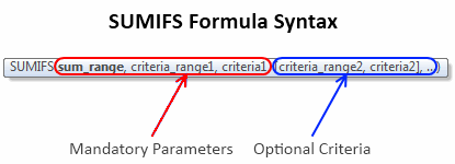
SUMIFS function – Syntax and explanation:
SUMIFS formula takes a range for summing the values and at least one criteria range and criteria. You can specify as many as 127 conditions for summing your data.
Imagine asking “how many spit bombs Hansolo sold in North region of Planet Naboo between long long ago and long ago that resulted in more than 25% profits?” and getting an instant answer.
The beauty of SUMIFS formula is that it works with wildcards too, just like its siblings – SUMIF and COUNTIF. So you can write formulas like,
=SUMIFS(D3:D16,B3:B16,"Spit Bomb",C3:C16,"*th") to get sum of spit bombs sold in North and South.
Using SUMIFS() with tables
You can write SUMIFS function on either a range of data or on a table. When using with tables, you can simply apply structural references – ie TableName[Column Name] notation to specify the criteria columns. See this example:

SUMIFS Examples
Let’s say you have a table named ACME as pictured above. See these examples to understand how the function works.
- Sales for Blow Torch in West
=SUMIFS(acme[Sales], acme[Product], "Blow Torch", acme[Region], "West")
- Total Sales above 150 in East
=SUMIFS(acme[Sales], acme[Sales],">150",acme[Region],"East")
- Sales of North for all excluding Pod Gun
=SUMIFS(acme[Sales], acme[Region],"North",acme[Product],"<>Pod Gun")
- Sales of all products that contain letter B
=SUMIFS(acme[Sales], acme[Product], "*B*")
Using SUMIFS() with Date & time values
When you have a column of dates, you can apply special operators like >, <, =, <> to specify a date range.
For example, to count total sales between March 2018 and May 2018, we can use
=SUMIFS(acme[Sales], acme[Sales Date],">=1-Mar-2018", acme[Sales Date], "<=31-May-2018")
You can either type the date in the formula or bring it from a cell. If you have two cells containing start and end date for your window of dates, you can use this formula.
=SUMIFS(acme[Sales], acme[Sales Date],">=" & start_date_cell, acme[Sales Date], "<=" & end_date_cell)
Replace start_date_cell and end_date_cell with actual cell references or names.
Bonus:
Just like SUMIFS, there is COUNTIFS and AVERAGEIFS too in Excel. Once you know SUMIFS(), you can use all these other functions with ease.
SUMIFS Examples – Sample Workbook
If you want to learn more about SUMIFS function and practice the formula, download Free SUMIFS Example workbook. Play with the formulas to learn more.
Top 10 formulas for data analysis
Learning and using Excel formulas correctly is the key to success when it comes to your career as an analyst. If you enjoyed this post, check out my top 10 formulas for analysts page for more tutorials.
Additional resources on SUMIFS formula
Please refer to these other web pages as well to learn many uses of SUMIFS.
- SUMIFS and many uses [exceljet]
- SUMIFS syntax, examples and best practice [Microsoft documentation]
- How to use SUMIFS function [techonthenet]


216 Responses
Very useful, thank you!
Very useful
Must… force.. IT-department… to UPGRADE THIS SORRY MESS TO Win7 & Office 2010!!!
*drooooooool…..*
I’ve been working with sumif formulas today and have been wondering how I can use 2 criterias or more. I have been reading about Dsum and Daverage. But, of course, this is much easier.
So thanks!
Of all the tips you’ve posted thus far, I can’t think of one that will be more beneficial to me in my day-to-day. Wanting to include multiple criteria in my SUMIF formulas has long been a serious point of frustration.
Question: How will this formula be handled by the conversion tool if someone opens my 2007 file with and earlier version of Excel?
Thanks for sharing, Chandoo.
I use these formulas a lot. I hope 2010 adds a bunch of additional ones. Don’t forget that the criteria can be referenced in from cells outside the formula. This is really helpful for building a summary table. As an example of the versatility of the formula, using Chandoo’s table, this formula =SUMIFS($C$2:$C$15,$A$2:$A$15,A2,$C$2:$C$15,F7) give a sum of 509 when the criteria value in A2 is “Pod Gun” and the criteria value in F7 is “>130”. Also, wild cards can be used in the criteria formula… setting the “A2” cell reference to “*un” yields the same result.
The astrick argument is gold. Saved me. Thanks Bill
thanks sir for giving much idea about sum ifs
Thanks for a hint. I fail to understand how this >130 logic is applied in this table? I mean, how do you put in SUMIFS formula? I would be thankful if you can give me whole formula.
@Ducheznee: Thank you. When you save a file with SUMIFS and open it in Excel 2003, the cells containing SUMIFS should show #NAME error (as the sumifs formula is not available in those versions). You can use one of the other methods (like SUMPRODUCT http://chandoo.org/wp/2009/11/10/excel-sumproduct-formula/ or SUM array formula http://chandoo.org/wp/2009/07/22/sumif-with-multiple-conditions/ ) to handle such cases.
@Bill.. thanks 🙂
@Jan Hogh: Totally agree with you. After using Office 2010 and Win 7, I dont feel like looking at windows xp comps.
@Cuboo and Finnur: Thanks 🙂
sir how can know sale of north and east
Use Pivate Table
Sumifs function is really working fine and thanks for the classic example.
Could you pl help me to understand ,how far it is differ from pivot table?
You know it’s funny. When Excel 07 came out, I found I had to stop using SUMIFS because so many people were still using 03, but then you rescued me with SUMPRODUCT Chandoo! =)
Hi and 100 more
as usual very impressive and cool especially with win7+office2010
Many Thanks
What could be reason for not moving to Excel 2007+ as even large multinationals are also stuck with Excel 2003 when nobody has any doubt about their superiority over previous versions. So what might be the reasons behind this reluctance to adopt this much better product over an obsolete and less relevant in todays environment even by large multinationals?
The larger the corporation the more applications are embedded and the easier it is to break things by up-editioning. Induhviduals can fix broken logic however when you have 35,000 computers introduce errors jumping to the next version (no matter how great it is) ALWAYS get me reaching for the hoiday booking form!
more and more i am using SUMIFS rather than VLOOKUP. it’s invaluable when you want to supply multiple criteria in a table that has more than one or two dimensions. of course you have to make sure that each table entry is unique.
I am a teacher and need some help….how do I create a multiple sumif formula:
I want to count/sum scores if they meet two criteria: Quiz and >=0
If a student is Absent “A” I dont want it to affect their average. Any insight on an easy fix would be great. Thanks!
Use COUNTIFS / SUMIFS
and AVERAGEIFS
@ bill – you just saved me a TON of time! I hope I will pay it forward on your behalf. Thank you.
Hi, Iam preparing a salary bill of an employee for a period form July-2008 to June-2010. In this mean time he got promotion on 18-01-2009. From that day his salary hiked from Rs.10030 to Rs.10565. He got one increment on 18-01-2010. That day onwards his salary again enhanced from Rs. 10565 to Rs.11115. I prepared this bill in excel-2007 worksheet. I wish to split the salary in the months when he got hike in his salay, with excel formulas. But I am unable to do it. Can ypu help me please?
Being first time in chandoo.org i loved it sooooo much … i become a great fan of chandoo cos its so simple and huge knowlege giving sites i have ever seen ..thanks a lot man ..god bless you
Hi Chandoo,
I’ve been following Chandoo.org for some time now. Great work!
Slight query regd. this post-
I’ve used SUMIF\SUMIFS in the past, but I do have one grouse. The need for putting criteria in double quotes means I can’t pull criteria from a cell reference which would make it much more powerful. i.e., instead of criteria “>150” how do i use criteria >$A$1 ? Some help please?
Thanks, Anish
@Gouse.. you can use SUMIF or SUMIFS to sum all the salary amounts prior to promotion etc.
@Jawad: Thank you 🙂
@Anish: you can simply type >150 in A1 and then use that in formula like =sumifs(range, a1). If you cannot do that, you can use B1 to concatenate A1 with the operator you want.
Hey Chandoo,
Thanks for that tip, Just tried it and it works! Nice!!
Thanks again!.
Anish, I am sure you did understand the side trick Mr. Chandoo showed you. But, a poor novice with this function like me, could not assimilate his trick. will you please be kind enough to show me in detail, or the actual formula you used? because, I am still fumbling with placing >150 in the formula!! Thanks a lot.
@Hirendra
The format of Sumifs if
=Sumifs(Sum Range, Criteria Range1, Criteria1, Criteria Range2, Criteria2 …)
=Sumifs(A1:A10, B1:B10, “>100”)
will sum A1:A10 where B1:B10 is > 100
or
=Sumifs(A1:A10, B1:B10, “>”&C1)
will sum A1:A10 where B1:B10 is > C1
useful thank a lot but if u could more examples as a challenging i would be much better
Hi Chandoo,
Excellent review of the new SUMIFS function!
Regarding the catch you mentioned above…
If you want to send Excel files to users of previous versions you must convert SUMIFS. To make Excel 2003 users see results instead of an error the user must use SUMPRODUCT or Array formulas.
This formula: =COUNTIFS(‘Sales’!$A$4:$A$400,”JAN”,’Sales’!$V$4:$V$400,1)
Turns into this one: =SUMPRODUCT((‘Sales’!$A$4:$A$400=”JAN”)*(‘Sales’!$V$4:$V$400=1))
This link may help:
http://www.excel-spreadsheet-authors.com/sumif-multiple-7-ways.html/
I am trying to reuse the same criteria range but different criteria using SUMIFS; however, after establishing the first criteria range and entering the same for the second criteria range the result is zero. Is there a structure to reuse the same criteria range or include more than one criteria with the first criteria range? The data source structure is static but the values always change and I need to compare two data sources by sum.
@Tuttler… Can you give me an example of what you are trying to do. I am unable to visualize your problem.
The basic structure I tried using SUMIFS is: =SUMIFS(C:C,A:A,”Value A”,A:A,”Value B”,etc…). In order to get the result of using the same set of criteria_range, I used: =SUMIF(SUMIFS(C:C,A:A,”Value A”),SUMIFS(C:C,A:A,”Value B”),etc…)). Other criteria was used within each SUMIFS to further define the specific data set needed. Depending on the number of items required from the criteria_range the formula gets cumbersome.
Hi Chandoo – great site! To follow up Tuttle’s question, let say I wanted to determine podguns sales in the North AND the South.
One way to try is maybe sumifs(podguns in the north) + sumifs(podguns in the south) although that might get cumbersome, I wonder if it might make more sense to try a dsum instead? I’m still in awe of / a little afraid of array functions {} but maybe you can use one as well?
Ravi
Hi,
Maybe you can help with a problem.
I want to use sumifs to calculate sums based on 1 criteria being today’s date.
I am using the =Now() formula to automatically update the date. However, it is not summing. If i replace the =now() with a hardwritten date, it works.
Any suggestions?
Thanks,
@Harris,
try using =Today() instead of =Now()
Today = Date
Now = Date and Time
Dear Chandoo
Sumifs work great,
but there is one short coming, one column one criteria
I cannot get sum of two different months
SUMIFS(Value,A19:A151,”April”,A19:A151,”May”)
Sumifs gives a “0” when i put a second criteria
I want to sum the sales of multiple/few months, the months are in Column A
ie one column multi criteria
Please Help
@Johnson Mathias
This is a short-coming in your logic not in Sumifs functionality
.
A cell in A19:A151 cannot be both April and May which is what you have asked Sumifs to do
.
Your query should be like
=SUMIFS(Value Range,A19:A151,”>”&DATE(2011,4,1),A19:A151,”<"&DATE(2011,5,30))
.
Give that a go
why is that Sumif, sumifs, or sumproduct formulas not automatically update unless the source file is opened.
They work fine same workbook but when external data source is involved it only work when source file is open.
Please help help help!!!
@Uzair
There is a good article at Daily Dose of Excel on this which is worth a read
http://www.dailydoseofexcel.com/archives/2004/12/01/indirect-and-closed-workbooks/
.
The comments also add other options
.
ps: There is no need to post here and in the Forums, they all get read
Hui,
I have a similar issue than 27), but I’m trying to have the criteria “Date” as a variable referred to in two separate cells. So I can define date ranges as I need.
Sumifs gives a “0? when i put a the criteria
Please help!
@Matias H
You can use something like
=SUMIFS(B19:B151, A19:A151, ”>”&D1, A19:A151, ”<"&D2)
Where D1 and D2 are the dates you want
Thanks so much!!
Using Excel 2007 I have changed and now almost exclusively use SUMIFS, its easier, and doing multiple criteria is quicker. I can track Date, Country, Dustributor and on and on easier with SUMIFS, that using SUMPRODUCT.
Hi Chandroo (or whoever can help me! 🙂 )
I need help – am very new to more advanced calculations in excel.
My problem: I want to use ‘sumifs’, however the cells I want to add to the “sumrange” are not together (i.e.: c10+c6+c2+d2+e2) and want to include the conditions of sum only when c10 is not 0. I continue to get an error when I put this formula:
SUMIFS(C10+C6+C2+C2+E2,C10,”0″) and off course an error when I put the full formula I want which is something like this: SUMIFS(C10+SUMIFS(C6+C2+D2+E2,C6,”0″),C10,”0″)
Any help will be very much appreciated!
EA
@EA
=IF(C10<>0,SUM(C2,E2,C6,C10),0)
Thanks a lot Hui! 🙂
I’ve reached the limits of my logic & after an hour of fiddling & researching have nothing to show for it.
How do you select multiple criteria in a criteria range? Column A has sales person name, in some cases I need to sum together more than one sales person.
When you enter the same range for both Criteria_range1 & 2 the result is 0. I’ve played with = combinations which works but is incorrect as Excel thinks I’m after a range.
In effect what I want to do is:
=SUMIFS(WEBI_LY,WEBI_BDM,”fosters group”,WEBI_BDM,”sean crowe-maxwell”,WEBI_BRAND,C3,WEBI_BUNDLE,D3)
Many thanks in advance guys!
@AP
Your trying to do this:
=SUMIFS(B2:B11,A2:A11,”a”,A2:A11,”b”)
What that says is Sum Column B when Column A = “a” and Column A = “b”
A single record can only be one or the other it can’t be both
.
You need to use something like:
=SUMIFS(B2:B11,A2:A11,”a”)+SUMIFS(B2:B11,A2:A11,”b”)
.
In your case
=SUMIFS(WEBI_LY, WEBI_BDM, ”fosters group”, WEBI_BRAND, C3, WEBI_BUNDLE, D3) + SUMIFS(WEBI_LY, WEBI_BDM, ”sean crowe-maxwell”, WEBI_BRAND, C3, WEBI_BUNDLE, D3)
this exercise would be easily solved if Excell had an “or” function as in ”fosters group” or ”sean crowe-maxwell”. But assuming this is not the case, how do you solve this if instead of the above 2 conditions, there were 5, or 6? the function would indeed be long, tedious and prone to errors. In other words, what I’m really looking for (as well as other users I suppose) is a filter to be expressed as a function. Last but not least, very valuable posts.
@Fred
You can do this in one formula using Sumproduct
=SUMPRODUCT(((A2:A11,”a”)+(A2:A11,”b”)),B2:B11)
The + is effectively saying or
so Where A2:A11 = a or b sum B2:B11
Hi Hui,
I have a similar issue and wanting to know if you can use SUMIF with Text Columns.
Col A Col B Col C
ProductName machineName Status
MS Office Desktop1 In Use
MS Office Desktop2 In Use
MS Office Desktop3 Removed
Want to sumifs for ProductNames installed on various machines with a particular status
Tom
@Tom
Can you post your file with some sample queries that you want to reproduce?
@Hui | Thanks mate! Had that as my work around whilst awaiting a response here, was just hoping for something a little cleaner. All cool!
excellent-the example really helped
Hi All,
trying to resolve this, i need my criteria 1 to be equal either 4 or 5. The logic is correct, just not returning the results
SUMIFS(E6:E108,C6:C108,AND(4,5),I6:I108,A122)
Thanks in advance
@Jackie
I hate to disappoint but the logic is a little bit out
What you have asked for is that a cell in Range C6:C108 has a value of 4 and 5, which a cell obviously can’t have.
And/Or aren’t really suitable for use like this, although at first glance it does seem like they should be.
.
I’d recomend the following:
=SUMIFS(E6:E108,C6:C108,4,,I6:I108,A122) + SUMIFS(E6:E108, C6:C108, 5, I6:I108, A122)
Hi, Is it possible to have the SUM_RANGE as a cell reference with the cell reference being a VLOOKUP formula result)?
For example: data downloads from another program each month into sheet 1, with month 1 in (say) col D, month 2 in E etc. so it grows column wise each month. In sheet(2) is a table of 12 months with corresponding column references ( cell a1 has 001.2011 and cell b1 has “D:D” , a2 has 002.2011 and b2 has “E:E”. In sheet 3 Z1 is a list ( being a1 to a12 dates. In Z2 is a Vlookup formula which looks up the relevant column reference (ie list choice 002.2011 gives “E:E” in Z2. In cell Z8 is the sumif formula : =SUMIF($A:$A,”wotnots”,Z2). This should look at col A for wotnots and choose col E (month2).
The cell accepts the formula but doesnt give a numerical result. Iam wanting to be able to change sumif parameter using list choice.
Hi,
This related to Excel 2007. I have a sheet with multiple columns. Column B has dates (dd-mm-yyyyy) ranging from 1st to 31st of the month depending on the month. Column H has the amounts I want to sum when they are greater than zero. Each date can have multiple rows so the totals row is dynamic but the column rows are generally static.
I want to sumif on the Column B values (day less than 25th) and Column H, as indicated, for values greater than zero.
So far, my formula which sits a few rows below the total in Column H is not working:
=SUMIF(B6:B164;VALUE(LEFT(TEXT(CELL(“contents”);”TT MMM JJJJ”);2))”<25";H6:H164)
I've stripped it back but the quotes seem to be giving me headaches? Any ideas?
Kind regards,
Philip
does it have to be a sumif? how about a sum with ifs and curly brackets?
=SUM(IF(TEXT($b$6:$b$64,”dd”)*10,$h$6:$h$164))))
then hit ctrl shift enter for the array curly brackets?
Ravi
Hi Philip
Regarding post 44) Philip November 21, 2011
Your table seems to be A6:H164
Try
=SUMIFS($H$6:$H$164,$B$6:$B$164,”0″)
Works like a charm
part of formula above is getting edited as HTML
SUMIFS($H$6:$H$164,$B$6:$B$164,”=25-11-2011″,$H$6:$H$164,”=0″)
Change the = signs with greater than & less than Signs
Dear Ravi and Johnson,
Many thanks for your responses. Uhnfortunately, I’ve been too busy to try them out but as soon as I do, I’ll let you know. @Ravi: I don’t see where your formula is checking that the B column value is less than 25? Whether it is a SUMIF is for me secondary. It just has to before the logic I explained. Note that as I explained the 164 value is dynamic (in my fomula I actually use the “row()- 1” instead of 164. I just put the 164 to reduce the number of brackets.
@Johnston: only the 25 (day) is static, the month and the year change.
how i can do sumif function in excel with tow condition in the same criteria, for example: sumifs of any rang with condition 4=< X <=6 .
thank you.
Hey Philip
I did not realize the day is static 25
One solution would be to add a Say “J” column called “Day” =day(B1)
Thus you get a usable day criteria
SUMIFS($H$6:$H$164,$J$6:$J$164,”=25?,$H$6:$H$164,”=0?)
Change the = signs with greater than & less than Signs
I hope this helps
To those wondering how to use an operand with a cell reference (and to the extent it wasn’t already posted) you simply concatenate the operand in quotes with the cell reference using an ampersand. So if your condition is less than or equal to the contents of C5, you type:
“<="&C5
Hui, you seem to recommend summing the result of two SUMIFS with slightly different criteria to satisfy the need for what is essentially an OR() function. Can you use an AND() or an OR() as a condition, or is yoru solution the only way to accomplish that?
My third and final post today: I answered my own question using Hui’s comments above. To satisfy an OR condition (such as numbers between two values) you just repeat the range to be evaluated twice, once with a “>=” condition and once with a “<=" condition.
Also, gotta give the obligatory shoutout…Chandoo's great!
Is it possible to use a cell reference in the range and sumrange in a sumif? I would like to type the sheet I want to reference in a specific cell and have the sumif formula reference that cell for the sheet information.
Misty, I use sumifs whose source data is on a different sheet all the time, I’ve also done it across workbooks. I’m not sure what you’re using the spare cell for as a reference though. Can you give an example of what you’re doing? I don’t want to give an overly wordy and unhelpful reply.
Hi Chandoo!
I have a problem….I have an Excel 2007 Sheet with Name of Dealers in Rows and Month wis Sales in Columns (Apr.10, Apr.11, May.10,May.11….Mar.11,Mar.12). I have a Dashboard Sheet where the user enters the starting month & ending month for e.g. Apr.11 TO Sep.11.
I want to calculate the No of Dealers having registered some sales in the period i.e. Apr.11+May.11+…..Sep.11 should not be Zero. This needs to be calculated dynamically depending on the value entered in the Dashboard Month Field.
@Vineet
No need to double post.
This has already been answered in the Forums
http://chandoo.org/forums/topic/counting-no-of-rows-with-non-zero-totals-over-non-contiguous-columns-dynamically
Hi Chandoo
Great explanation of SUMIFS. But for summing up the values where data are spanning across multiple columns (e.g., data in 23 columns D:Z), is there a simple way? One could always write the SUMIFS statements for each column, using multiple criteria (e.g., criteria in 3 columns A:C), and then combine the results through simple addition, but this is not very elegant and in this case would require addition of 23 terms rather than one.
For example, this sums one column (and could be repeated, tediously):
=SUMIFS(D2:D10,A2:A10,A1,B2:B10,B1,C2:C10,C1)
but this returns and error, rather than summing 23 columns:
=SUMIFS(D2:Z10,A2:A10,A1,B2:B10,B1,C2:C10,C1)
Thanks for your input and help.
Sorry, but I had mistyped my email address a minute ago (linked to my question on using SUMIFS across multiple columns). This time it is correct.
Wow, great time saver. Thank you. I used it for the wildcard with the sumif.
Normal
0
false
false
false
EN-US
X-NONE
X-NONE
/* Style Definitions */
table.MsoNormalTable
{mso-style-name:”Table Normal”;
mso-tstyle-rowband-size:0;
mso-tstyle-colband-size:0;
mso-style-noshow:yes;
mso-style-priority:99;
mso-style-parent:””;
mso-padding-alt:0in 5.4pt 0in 5.4pt;
mso-para-margin:0in;
mso-para-margin-bottom:.0001pt;
mso-pagination:widow-orphan;
font-size:11.0pt;
font-family:”Calibri”,”sans-serif”;
mso-ascii-font-family:Calibri;
mso-ascii-theme-font:minor-latin;
mso-hansi-font-family:Calibri;
mso-hansi-theme-font:minor-latin;
mso-bidi-font-family:”Times New Roman”;
mso-bidi-theme-font:minor-bidi;}
Is there any way to get SUMIFS to do either/or criteria?
I was only able to get it to work with an array constant:
=SUM(SUMIFS(sum_range,criteria_range1,criteria1,criteria_range2,{“A”,”B”,”C”}))
However, arrays constants can’t use references like F1,F2,F3.
Is the ONLY alternative to use SUMPRODUCT (much slower) or to use multiple SUMIFS (very long formula and high maintence).
Lawrence
Yikes…what happened to my post?
How do I edit out all that code???
~L
Thanks, if everything was explained like this, everything would be easier to understand and do.
works just great, but I need to add an ampersand & to it to concatenate:
=SUMIFS($D$2:$D$15,$B$2:$B$15,”bli”,$C$2:$C$15,”>”&50)
Without the ampersand does not work at all with = or > or >=, just with a number. No matter if I put that in single or double or without marks. But with & works nicely. Sure I will use the sumifs quite some times.
So that would make Sumproduct the

of Swiss Army Knives
give some more range.
I do stuffs like this in MS Excel 2003 by using the sumif + concatenate function. Where concatenate resides in new column. =sumif($A$14:$A$27,”Pod GunEast”,$C$14:$C$27) where Column A is concatenation (&) of Column B and C.
Its very Helpful!! thank you
Hey Chandoo, you are really awesome!! Now I will use sumifs instead of sumproduct!
Thanks a million!!
Hello There. I found your blog the usage of msn.
This is a very neatly written article. I’ll be sure to bookmark it and return to learn more of your helpful information. Thanks for the post. I will certainly return.
Thanks Chandoo. It was very useful. No need to make a Pivot.
Is there any reason why a sumif statement will not work on a text cell with a < or > symbol in it? I’m using these symbols to put data into buckets: >12 weeks, >26 weeks.
Cell A1: >12 weeks
=SUMIFS(Value to Sum,criteria range,A1)
=0
Am I stuck with changing all the text to ranges: 12-25 weeks, 26-52 weeks?
@JustiinCBU
Can you post a sample file, Refer: http://chandoo.org/forums/topic/posting-a-sample-workbook
dear sir,
plz help formula us to 2003
sumifs in summary sheet
me formula is
sumifs(‘sheet 3 (cell s:s(value),’cell e:e(div),’summary sheet1 (cell c5 (ctv),'(sheet3(cell aa(status),summary sheet1 (cell c8 (applied),'(sheet3(cell k(month),summary sheet1 (old)
@Anil
Can you post a sample file, Refer: http://chandoo.org/forums/topic/posting-a-sample-workbook
Thanks Chandoo
Your excel tips r really awsome & making us awsome.
Can anyone help me out in this following condition:-
Suppose I want to make different sales sheets each of Pod Gun, Blow Torch & Spit Bomb. Is it possible that as I type the entry in general table (containing all products), the entry also goes to its respective excel sheet ?
Would b thankful
What if you want one of the criterias to pull from whatever is in a particular cell to the left?
Right now my last criteria is unique customer names that I have to type, but I would rather the last criteria be a cell reference so that I can just drag the formula down.
Hey Ella, see my posts above for using cell references and creating or conditions. I pasted one of them below:
“To those wondering how to use an operand with a cell reference (and to the extent it wasn’t already posted) you simply concatenate the operand in quotes with the cell reference using an ampersand. So if your condition is less than or equal to the contents of C5, you type:
“<=”&C5 “
we can also use sumproduct same a sumifs right????
Dear Chandoo,
I don’t have my own business neither appointed at a prominent position, despite of these shortcomings i’ve designated as “CEO” in the organization i’m employed at, and i acknowledge that its just b’caz of people like you. I’m fortunate to have you.
CEO = Chief Excel Officer
Wish you all the best!
Thanks.
It is really very good and helpfull!!!
Great Chandoo…. 🙂
Question for you Chandoo, and maybe it is already addressed somewhere in the dialogue above.
Can the “SUMIFS()” formula fully replace the ARRAY formula that looks up criteria in multidimensional ranges? For example, I have the table below, I would like to search by Dept, Employee, Type, and then horizontal for a specific month. I cannot get the horizontal sum-if function to work.
The following formulas return #VALUE!, but of course works when I change the sumrange to equal a specific month column.
=SUMIFS($D$2:$F$5,$A$2:$A$5,”Sales”,$B$2:$B$5,”Mary”,$C$2:$C$5,”Contract”,$D$1:$F$1,”MAR”)
A
B
C
D
E
F
1
Dept
Employee
Type
JAN
FEB
MAR
2
Finance
John
Contract
160
160
160
3
Sales
Bob
Full-time
195
180
185
4
Sales
Mary
Contract
155
150
170
5
Sales
Fred
Full-time
165
155
150
I’d like to replace the cumbersome ARRAY formulas in my worksheets now that I have 2010, but the new SUMIFS formulas still seems to be limited in comparison (although it is much easier to understand).
Hey, great article and illustrations.
This YouTube video is also good to see the sum, sum if and sum ifs functions in action – youtu.be/pYdOukeuENQ?a
Sir….Brilliant tutorial with illustrations….and u r SuperBrilliant.
Its a pleasure to watch ur vids.
Blessing$.
Great use of * i learnt today
Hi,
Im having a problem with my SUMIFS formula. At the moment my formula looks like this =SUMIFS(‘Booked ‘!$H:$H,’Booked ‘!$F:$F,”>=”&$C$4,’Booked ‘!$F:$F,”<="&$D$4,'Booked '!$A:$A,$A8) This is looking up cancellation values within a certain date for a specifc sales person and is working fine. I now need to to add a criteria which will be the cancellation reason (the value of a specific cancellation reason) but i cannot figure out how to do this? everything keeps on coming back with a value of 0?
Please help???
@Edd
Simply add another range and criteria
eg: =SUMIFS(‘Booked ‘!$H:$H,’Booked ‘!$F:$F,”>=”&$C$4,’Booked ‘!$F:$F,”<="&$D$4,'Booked '!$A:$A,$A8, New_Range, New_Range Criteria )
Note that the Range must be the same length as the previous ranges
Posting a sample of the new formula and it';s criteria will assist us to help you further
Thanks for that but im still getting a value of 0. I am looking up data on the same summary sheet but from a different tab so this is what my formula looks like when it works =SUMIFS(Cancelled!$H:$H,Cancelled!$F:$F,”>=”&$C$4,Cancelled!$F:$F,”=”&$C$4,Cancelled!$F:$F,”<="&$D$4,Cancelled!$A:$A,$A8,Cancelled!J:J,E7) it comes back 0. What am i missing?
Thanks sooo much for your help!!!
@Hui
Sorry that didnt copy correctly,
Forumla that works =SUMIFS(Cancelled!$H:$H,Cancelled!$F:$F,”>=”&$C$4,Cancelled!$F:$F,”=”&$C$4,Cancelled!$F:$F,”<="&$D$4,Cancelled!$A:$A,$A8,Cancelled!J:J,E7)
@Edd
Can you post a sample of your file
Refer: http://chandoo.org/forums/topic/posting-a-sample-workbook
Hi Chandoo,
I had a query regarding the SUMIFS formula…while defining the criteria for a given range, can i type the criteria in the formula instead of giving cell reference? I tried putting the criteria in quotes (tried both ‘X’ and ”X”…but excel is showing error in formula…Could u pls help me on this?
hi,
I just started to learning sumifs which is a great tool to use. I have a problem here and I need help.
My data consists of salary and benefits details for professional staff, support staff, NBD staff & Management staff for both Singapore & Australia. I need to split total cost between:
1. professional staff / Singapore – I got the answer for this since there’s only 1 criteria
2. Support/NDB/Mgmt staff / Singapore – i got a nil answer when I did this….
SUMIFS(‘Cost report I’!AH3:AH43,’Cost report I’!C3:C43,’Cost summary’!A4,’Cost report I’!D3:D43,”Supp”, ‘Cost report I’!D2:D42, “NBD”)
I got the total cost for support staff but when i tried to add NBD….it gives me nothing. Can anyone enlighten me please.
thanks
@Mary
Check that the cells have “NBD” and not ” NBD” or “NBD ” etc
The spaces will confuse things
thank you for your quick reply Hui. I just corrected the space but it is still not picking up the total cost.
Can you email me the file at ihuitson at gmail dot com?
I have been using the SUMIFS formula to build a payroll Sheet for our office, however I track the hours in one sheet along with the days of the week and the specific job numbers, I then have another sheet that has all of the relevant employee information such as employee number and craft code, finally, I merge all of these onto a landing page where I am using combination VLOOKUP Formulas to auto-fill the needed information and then use dates and the top of the sheet in order to tell which week I am getting the information for. Now the SUMIFS are used in the hours columns to total all of the hours that the employee worked on the above date, and the specific job #, however as new employees come on and I add them to the list, it is no longer in alphabetical order, so when I use the filter buttons that are atop my sheet, It re sorts alphabetically but the formulas mess up and start referencing their old location even when they are unlocked or locked? Help Please?
I do not remember clearly when it was the first time when I came across Chandoo’s excel tips site – maybe in 2009, and thanks to the visuals and enjoyable diction, I am sure I will always remember the name Chandoo and will be able to come back to find the awesome solutions to my excel questions.
Thank you, Chandoo! 🙂
Question: In the illustration above, how do i write a formula if i need the number of Pod guns & spit bombs sold in the North??
Is it possible to find out the number of both Pod guns & Spit bombs sold in the same formula?
Hi Chandoo,
Couple of days back I got to know abt ur website thro a link. Amazing place to learn excel. found it realy help full. I have a question the in the sumifs formulae above, I want to find out the “Split Bomb” total for Both “North” and “West” region how do I find. I used the same sumif formulae with a {} to inuput North & West but its not working. Can u please help me
very nice tips ….
I like it
I learn some thing from it
i dont know how to use the downloaded excel workbooks that when downloaded are in xml format. Can you please tell me how to open them?
hi,
i am using SUMIFS to reference to a seperate workbook (a timesheet)
the formula figures out how many hours (entered) people did within specific date ranges. (creating a large consolodation spreadsheet).
the problem is, when trying to update the references, all i see is #VALUE! unless i open up that specific sheet it is trying to reference to.
is there a way for this formula to auto update? i read somewhere it needed =sum(ifs(————)) but this doesn’t work for me.
any help is appreciated!
@Ben
Is Calculation set to Automatic ?
Pressing F9 will recalculate the worksheet
@Hui
thanks for your reply. It is set to automatic and have tried manually recalculating. as soon as the external sheet is closed and i try to recalculate it comes up with #VALUE!
I have since read on microsoft help (http://www.mrexcel.com/forum/excel-questions/448762-value-error-sumif-external-link.html) that “SUMIFS” cannot automatically reference from closed sheets. SUMPRODUCT(s) is needed instead to update automatically. I need to figure out how to convert my SUMIFS SUMPRODUCT(s) now! :S
I, have this problem: I need to find a function for each row of the data D2: I17. If the condition A2 = 1 + mount & year = equal; sumproduct (all 1 of range D2: I17). col B Col C and unique data . Thank you.
A B C D E F G H I
CRIT Mounth Year v1 v2 v3 v4 v5 v6
1 January 2015 6 15 12 9 5 2
2 January 2015 10 4 7 15 14 13
3 February 2015 7 16 6 15 12 13
4 February 2015 6 11 11 12 12 2
5 March 2014 5 5 15 15 8 4
6 March 2014 1 6 8 6 16 6
7 April 2014 1 13 1 9 4 2
8 April 2014 3 2 9 15 14 2
9 May 2014 1 15 9 5 2 4
10 June 2013 3 14 11 4 13 11
11 July 2013 6 3 3 11 8 13
12 August 2014 16 1 8 15 11 10
13 September 2012 12 15 2 15 10 9
14 October 2012 8 7 2 14 5 9
15 November 2011 3 3 5 5 11 4
16 December 2011 3 3 10 8 8 4
Hi Michael,
Thanks for your question. I am not sure I understand this. Can you explain better? May be tell us what is the answer you are expecting for first row?
In Lotus 1-2-3, you can enter criteria into database functions and avoid the primitive criteria range that Excel still requires (last used in Lotus 3.0). I cannot fathom why Microsoft Excel developers haven’t changed the database functions so that they have this capability. I wonder if there is a way to communicate with them and express displeasure about the need for criteria ranges.
Chandoo you are the best!!!!
Thank you so much, it really helpful!!!
THANKS FOR IT.IT’S VERY USEFUL.
dear Sir.
I need you help , sorry I know my English is not good , so I have Main table it’ included Product and model . I need to make new table but product and Model not repeated together (look like primary key).
thank for you cooperation
Product Model
jeans Levis
jeans Levis
jeans GAP
jeans GAP
T shirt Levis
T shirt Buma
T shirt Gap
jeans Buma
jeans Gap
T shirt Buma
jeans GAP
jeans Levis
T shirt Levis
Product Model
jeans Levis
jeans GAP
T shirt Levis
T shirt Buma
T shirt Gap
jeans Buma
@Magdy
Select A1:B14
Then apply an Advanced Filter to the list
And extract Unique Entries to a different location without any filtering
HI TO CALCULATE THE SUM BETWEEN TWO RANGES.
That Is suM ALL BETWEEN 1000-5000
& 5000-10000.
The formula i am applying is Sumifs(B3:B990,”1000″)
@Akash
=Sumifs(B3:B990,”gt1000″,B3:B990,”lt5000″)
=Sumifs(B3:B990,”gt5000″,B3:B990,”lt10000″)
swap gt and lt for Greater than and less than characters
Very nice article. Thank you very much…….
Not sure if possible but I need to do a sumif for a headcount by region and department. The regions will be listed vertically on column A3:A15 while the departments will be listed horizontally A2:G2.
The issue is the departments are rollups with multiple departments falling into each rollup. Can I do a vlookup on the department to see which rollup it falls under and place that vlookup in a sumif?
I hope I am asking that clearly.
I am trying this out exactly as above (SUMIFS) in Excel 2010 and it is returning a ‘0’. Any thoughts? Pretty sure its user error.. 🙂
Man!!!!
you are my bro!!!
I work on servers and use excel only to vlookup and stuff. I told in an interview that I am an advanced excel user as job was related to hardcore data. I got the job and now I am learning the “advanced excel”
this was helpful
Thanks
🙂
Hi,
Good day!
Hope to be well.
I hereby inform to that, I was working as an assistant accountant, will need to Excel skills from basic to advance level now, so kindly provide me tremendous advice for how to improve those kind of Excel skills by myself.
Looking forward to your prompting response
Regards & Thanks
These are very helpful and make work easier. Thanks a lot for sharing the knowledge Chandoo.
Thanks & Regards
Shubam
I m big fan to chandoo.org b’coz chandoo logic is too simpla and work
This just saved me hours of work – thank you! You have a new fan!
Awesome. So useful. Thank you so much.
I am having a problem writing index formulas, I have a colum of names in A and a colum of numbers in F In another cell in E2 I want to input a number and get the closest 3 values put in 3 new cells with their corresponding names from the details in colum A.
Thanks for any help you can give,
All The Best
i owe you alot to this site to giving me chance to learn wonderfull formulas in excell
thank you….
Hi Chandoo,
how would you determine the “Sales of Pod Gun AND Blow Torch in North” using SUMIFS?
It seems like if we use multiple conditions from same column, it doesnt execute the right number, instead gives a 0!
Hi,
I would like to make the productivity sheet with the use of SUMIFS function in excel, so please give a advice to me, how can i make it?
nice
hi
i want to do sumifs, but one of my criteria range is in column and the other is in rows. i am giving my data and result what i am looking for.
Data is
Dept 101 102 103
505 209 333 315
501 209 155 261
532 144 166 257
43 110 187 257
43 326 232 218
45 232 352 236
499 167 235
185 61 41 76
185 61 41 76
185 33 43
185 33 29 43
185 55 41 66
185 61 41 76
and result what i want is
Dept 101 102 103
505 209 333 315
501 209 155 261
532 144 166 257
43 436 419 475
45 232 352 236
499 167 0 235
185 303 193 381
note that i have approx 100 such columns and thousands rows.
The data i get is from some other source and i cant use sumif because what if the column headers(i.e. 101, 102, 103 etc…) is changed in source data.
@Priya
Can I please suggest that you post the question at the Chandoo.org Forums
http://chandoo.org/forum/
Please attach a sample file as it is confusing to decode this text
You may also want to read:
http://chandoo.org/wp/2011/05/26/advanced-sumproduct-queries/
The way I’ve solved it is with =SUMPRODUCT(). The syntax is: =SUMPRODUCT(((CRITERIARANGE1=CRITERIA1)*(CRITERIARANGE2=CRITERIA2)*(CRITERIARANGE3=CRITERIA3)…),SUMRANGE)
The trick is to make sure that the sum range is a range of cells contained within the criteria ranges (that is, if you have criteria in cells C3 through AB3, and another criteria in cells B11 through B50, your sum range needs to be C11:AB50)
If the ranges don’t line up you should get a #VALUE! error.
@FG
Thats correct
You can read more about this style of use of Sumproduct at:
http://chandoo.org/wp/2011/05/26/advanced-sumproduct-queries/
thanks a lot, its working :):)
Please help me Need formula to grade the agents based on two criteria
Condition Male Female
>400 A+ A
>300 A B
>200 B C
>100 C D
SL NO Marks Grade
1 Male 500
2 Female 200
3 Male 357
4 Female 307
5 Male 330
6 Female 387
7 Male 369
8 Female 324
9 Male 380
10 Female 100
@Manju
Can you please post the question in the Chandoo.org Forums
http://forum.chandoo.org/
Please attach a file so that a specific answer can be delivered.
This works great as long as the data never changes. But can anyone tell me how to capture the data and it accumulate as it changes? Example: I have data in column b2:b7 that changes based on data in column a2:a:7 that changes. I want to capture the data in column b and and sum it in cell c2 and d2 based on the conditions of a2:a7, and never lose the values. They should just accumulate.
@Hostile
Can you post the question in the Forums
http://forum.chandoo.org/
Please attach a sample file to clarify the requirements
HI,
Please send me a VBA learning notes .
Thank you.
Azeem
Nice Example..!!
I am using excel 2010 and can’t seem to get the array formula to work with CTRL+SHIFT+ENTER.
This is my data:
A B
1 37 3
2 350 4
3 350 4
This is my formula:
=SUMIF(C6:C8,”>1″,{B6:B8*C6:C8})
The result I want. The sum of column B, (A * B) where B is greater than one.
Thanks in advance
@Kylie
Try: =Sumproduct((B6:B8>1)*(B6:B8)*(C6:C8))
use a simple Enter
hi,
I am new to excel, can anybody please explain me, why, where and how? to use “&” while drafting a formula.
Thanks in advance.
@Abdulaziz
& is only used to join text or strings together
=A1 & A2
=”Hello ” & A1
=”Hello” & A1 & A2
etc
hi all
i was working on SUM, SUMIFS, wanted to sum the sales of two different regions. was able to get result in SUM but failed to get one in SUMIFS
thanks hui 🙂
I want to make data in excel file , ( Sheet 1= Summary data {like below ) , sheet2- join detail date wise , sheet 3 – left detail date wise ) in a week /month.
i want to total of join qty from sheet 2 in sheet 1summary data.
according to name of person.
and same thing want from sheet 2 left data
a another data also required batch code – which are available of balance qty.
Pl help .
Hi Chandoo,
I’m struggling with 2 formulas to use to get info from a variable set of columns, for instance I want to sum up all sales from week Jan 4th until Jan 18th for all Pod Gun
and second for all Blow torch, region west for weeks jan 18th – feb 8th
Input data:
Product Region 4-Jan-16 11-Jan-16 18-Jan-16 25-Jan-16 1-Feb-16 8-Feb-16
Pod Gun North 127 177 100 144 103 127
Blow torch west 139 170 127 172 168 139
Blow torch west 103 144 139 167 122 103
Spit bomb North 168 172 103 100 200 168
Blow torch North 122 167 168 127 177 122
Spit bomb west 200 100 122 139 170 200
Spit bomb south 177 127 200 103 177 177
Pod Gun south 170 139 177 168 170 170
Blow torch south 177 103 170 122 144 177
Blow torch North 170 168 177 200 172 170
Spit bomb west 144 122 170 177 167 144
Pod Gun east 172 200 144 170 100 172
Pod Gun east 167 177 172 177 127 167
Spit bomb east 100 170 167 170 139 100
Can you or someone help me with this one?
this can be done through pivot table option, I tried and see the outcome.
Product Region Sum of 04-Jan-16 Sum of 11-Jan-16 Sum of 18-Jan-16 Sum of 25-Jan-16 Sum of 01-Feb-16 Sum of 08-Feb-16
Blow torch North 292 335 345 327 349 292
south 177 103 170 122 144 177
west 242 314 266 339 290 242
Blow torch Total 711 752 781 788 783 711
Pod Gun east 339 377 316 347 227 339
North 127 177 100 144 103 127
south 170 139 177 168 170 170
Pod Gun Total 636 693 593 659 500 636
Spit bomb east 100 170 167 170 139 100
North 168 172 103 100 200 168
south 177 127 200 103 177 177
west 344 222 292 316 337 344
Spit bomb Total 789 691 762 689 853 789
Grand Total 2136 2136 2136 2136 2136 2136
after this you need to draw simple sum formula
Dear all,
I hv an issue, while using the Sumif Function & I could not find anything error.
SUMIF($B$1:$AJ$3132,AM13,AD:AD)
The Target result would be 59 , wherein the result is 61. Out of 6 places, 5 Places the result is right & only one Place the result is not correct.
LAst 3 days, I am breaking the Head to find out the right solution.
ANY feedback Pl.
regards,
K.G.Radha Krishnan.
@Radha
The length of the Sum Range must be the same as the Criteria Range
Try: =SUMIF($B$1:$AJ$3132,AM13,AD$1:AD$3132)
Hi i want to know how to calculate the total working hours for the weekdays only
Very nice formula.
I am too late to understand such formulas
very nice sir ji example
Hi
i am trying using sumifs by having criteria row and column but getting an error
please advise
@Sridharan
Try a Sumproduct Query
Refer: http://chandoo.org/wp/2011/05/26/advanced-sumproduct-queries/
Hello,
I know basic excel,
But , i want to be master in excel
Please send me mail from Basic……………
Or
Give me way to be master in MIS……Or Excle…
Subtotal with atl+shift+L is better option for easy calculation.
This is a great article. You are sharing valuable MS excel tips. As an accounting professional, I used SUMIFs formula for reports preparation. It is a good practice to use the Name manager function and SUMIFs together because it makes it much easier to remember.
very useful.
clearly explained
Hi
what i’d like to do is —- sum the value that meets multiple criteria from another workbook.
i use SUMPRODUCT formula and it works just fine in office 2010.
but now i am upgrading to office 365, and the formula no longer works.
(the same excel file but open in office 365).
please advise if there is any solution for this. BIG TKS
Very helpful to learn excel Thanks
This might be one of the blonde questions but I don’y know how to transfer/copy the data in the article above to Excel in order to practice what is taught about SUMIF
Hi
In order to practice is there a way I can copy the table to Excel or how do you guys doing it? Thanks
i want to learn about advance excel so if i flow the tutorial i will expert in excel or not…
Thanks for explanation. Very useful.
very insightful!
Great Info Sir
Hi Chandoo
Thanks for this, i use this often and never get tired…..
Thanks for sharing such a good article on excel SUMIFS Formula this site to giving me chance to learn wonderful formulas in excel. thanks for this and just keep posting
for sum ifs function,I want to calculate Function of One region only. how can i compute.
anuraag
9560731283
@Anuraag… what do you mean by calculate function of one region only?
Hi Chandoo,
Thanks for putting up the web-page on advanced excel learning tutorial. As I am planning to move on to a different role that requires me to be equipped in pivot table these lessons will be useful.
Hi All,
I have a unique problem with sumifs . I have 5 conditions/parameters for sumifs , out of which 3 conditions might have 1 / multiple selections (values coming from user selected multi list box and falling in different cells ) .ALL Conditions are Character variable .
In this case i have sum up spends value using sumifs for all possible combinations user will select from the drop down menu and i have to keep the parametrs automated (cell referenced – as they are user defined ) and i cannot hardcode them using {} .
How can i do it using SUMIFS .
Regards
Abhishek B
Hi Abhi,
Have you tried using Pivot Tables and slicers for this? They might be easier than SUMIFS and you don’t need to write any formulas. See this for an intro to slicers – Introduction to Slicers – What are they, how to use them, tips, advanced techniques & interactive reports using Excel Slicers
Hi
I have a question around SUMIF and INDEX MATCH MATCH
My INDEX MATCH MATCH formula is giving me the result for the one vendor i am doing a lookup but i want to do a sumif if there are multiple entries for the same vendor in the array.
https://answers.microsoft.com/en-us/msoffice/forum/all/sumif-and-index-match-match-formula-help/ec6c3c44-6c92-47ff-b909-ee3812843300
I have tried to explain this here in the MS community but i have not had any response
Thanks for help in advance
Nishesh from NZ
Hi,
Chandoo, You are doing a great job. but please can you translate your all lectures in simple Hindi. Further plz guide, are you lectures lesson wise available for new learner.
Regards,
Rizwan
You have a great site, I have found the site and formulas you have shared here very valuable. Thank you for taking the time to put this stuff together! I use the sumif function all the time and reference this page when I mess it up 🙂 Keep it up.
Hello. How come when I use the filter option then try to apply this SUMIFS(D10:D23, C10:C18, “West”) function I do not receive any outcome?
You have used “wrong ranges” for the formula.
Try this: SUMIFS(D10:D23, C10:C23, “West”)