
Situation
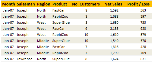
Not always we want to lookup values based on one search parameter. For eg. Imagine you have data like below and you want to find how much sales Joseph made in January 2007 in North region for product “Fast car”?
Data:
Solution
Simple, use your index finger to scan the list and find the match 😉
Of course, that wouldn’t be scalable. Plus, you may want to put your index finger to better use, like typing . So, lets come up with some formulas that do this for us.
You can extract items from a table that match multiple criteria in multiple ways. See the examples to understand the techniques:
| Using SUMIFS Formula [help] | |
| Formula | =SUMIFS(lstSales, lstSalesman,valSalesman, lstMonths,valMonth, lstRegion,valRegion, lstProduct,valProduct) |
| Result | 1592 |
| Using SUMPRODUCT Formula [help] | |
| Formula | =SUMPRODUCT(lstSales,(lstSalesman=valSalesman)*(lstMonths=valMonth)*(lstRegion=valRegion)* (lstProduct=valProduct)) |
| Result | 1592 |
| Using INDEX & Match Formulas (Array Formula) [help] | |
| Formula | {=INDEX(lstSales,MATCH(valSalesman&valMonth&valRegion&valProduct, lstSalesman&lstMonths&lstRegion&lstProduct,0))} |
| Result | 1592 |
| Using VLOOKUP Formula [help] | |
| Formula | =VLOOKUP(valMonth&valSalesman&valRegion&valProduct,tblData2,7,FALSE) |
| Result | 1592 |
| Conditions: | A helper column that concatenates month, salesman, region & product in the left most column of tblData2 |
| Using SUM (Array Formula) [help] | |
| Formula | {=SUM(lstSales*(lstSalesman=valSalesman)*(lstMonths=valMonth)* (lstRegion=valRegion)*(lstProduct=valProduct))} |
| Result | 1592 |
Sample File
Download Example File – Looking up Based on More than One Value
Go ahead and download the file. It also has some homework for you to practice these formula tricks.
Also checkout the examples Vinod has prepared.
Special Thanks to
Rohit1409, dan l, John, Godzilla, Vinod
Similar Tips
- Excel SUMIFS Formula – What is it, how to use it & examples
- Excel SUMPRODUCT Formula – What is it, how to use it & examples


63 Responses
=Index(RngToPick,Match(1,Conditions,0)) non array entered
Where Conditions is defined as For eg Conditions = ($a$1:$a$10=d1)*($b$1:$b$10=e1)
Having more than one match for the search parameter would render the VLOOKUP Formula and the INDEX & MATCH Formulas with a single total and therefore the wrong answer. The SUMIFS, SUMPRODUCT, and SUM array formulas would give the correct answer should there be more than one match.
Fantastic worksheet, by the way. Loved all the formulas.
It’s about time you stopped ignoring the DSUM function, Chandoo.
=DSUM(Database,”Net Sales”,criteria)
where:
* ‘Database’ is the named range $B$4:$H$1083 (i.e. all your records, including the column headers)
* “Net Sales” is simply the name of the column you are interested in adding up (and you could also use ‘6’, which would tell the column to choose the 6th column from the edge of your database range)
* ‘criteria’ is a range of 8 cells that list each column you will be filtering on in the first row, and the things you are looking for in each column in the second row, i.e.:
Salesman Month Region Product
Joseph Jan-07 North FastCar
I’ve uploaded an amended spreadsheet to http://cid-f380a394764ef31f.office.live.com/view.aspx/.Public/vlookup-on-multiple-conditions%20-%20DSUM.xls if anyone wants to play around with DSUM.
Also check out http://www.techonthenet.com/excel/formulas/dsum.php for more examples of DSUM
Hi everyone,
I have tried all of these options and none of them are working for me. I keep getting a #VALUE error. What am I doing wrong?
FYI I have a workbook with 4 sheets. I am using two sheets for this formula. This sheet that my data is in is called Fullyear (it has employee names in 1st col, then each employee has 6 different timeoff criteria, holiday, vacation, sick, personal, birthday, other listed in col 2, then the answer I seek is in the last column of the spreadheet named Endbal). The criteria to lookup is in sheet 4 called Lookup and they are in drop down format (so they should match), There are two criteria, employee name and timeoff so I choose “Joe Smith” and “vacation” and I want it to give me Joe Smith remaining vacation time from the last column.
Thank you
The link
http://cid-f380a394764ef31f.office.live.com/view.aspx/.Public/vlookup-on-multiple-conditions%20-%20DSUM.xls
Isn’t available
I know its been more than 10 years but Could you please send me the link of the spreadsheet on
hussain_786_23@yahoo.com
Thanks
The link works ok
When the Pop-up appears simply press Cancel and the File opens
can you also help me with finding the minimum of values based on multiple conditions.
@Praveen
Can you be a bit more specific like what conditions and what type of data and even ranges if you have them?
Hi Hui,
My requirement is to find a least cost option among various combinations for port transport.
My data table would have the name of source port, name of destination from port, type of vessel to be handled, cost of transportation (port+ inland and others).
I need to find the least cost for a specific destination for a specific vessel among various ports.
You can explain it using the data provided above in your example, instead of a specific output i need a min among the selection. Lets say lowest sales by joseph for fast car in your example.
I was able to get the solutions after burning some brain cells by applying pivot table. Is there any specific way to do this with cell formula.
regards
praveen
@Praveen.. you can use MIN() formula to do this:
For eg. Assuming A1:A100 has sales person name, B1:B100 has product and C1:C100 as sales and you want to find out what is the min. sales for John for the product ABC,
=MIN(IF((A1:A100=”john”)*(B1:B100=”abc”)=0,””,C1:C100))
You must enter this as an array formula – ie press CTRL+SHIFT+Enter when you finish typing to get the result.
Chandoo,
In the above scenario, for getting the Max sales, it was possible to do so without the use of an array function (as below). Wondering if it is also possible to get the min sales without the use of an array …
=MAX(INDEX(((A1:A100=”john”)*(B1:B100=”abc”)=1)*C1:C100,0))
Thanks,
Farhad
Hi Chandoo,
Firstly I want to thank you and also this forum. I learned a lot. I’m very appreciate.
I tried the below ones for create conditional min and max formulas. But I couldn’t success to make them run.
(My data is like exactly you define : A1:A14 has sales person name, B1:B14 has product and C1:C14)
=MIN(IF(($A$1:$A$14=”john”)*($B$1:$B$14=“abc”)=0;“”;$C$1:$C$14))
=MAX(INDEX((($A$1:$A$14=”john”)*($B$1:$B$14=”abc”)=1)*$C$1:$C$14;0))
(with press CTRL+SHIFT+Enter)
What is missing in these, i wonder?
May I ask your help please?
Thanks a lot in advance….
Hey praveen,
Check the Dsum formula given by jeff weir above…
Similarly, you can use Dmin formula to get Minimum value as per mutiple criterias
Database Functions -> Dsum,Dmax, Dmin, Davg etc r very easy n Powerfull without any Complex nested formulas.
fyi – Hit F1 in Excel & search Database Functions – You’ll get entire list with syntax n example
@chandoo…that’s funny, I thought I commented on this, but my comment didn’t show. Can you check your spam filter?
hi chandoo,
works wonderfully. I was not able to ignore the irrelevant values in my minimum function. “” this has done the trick.
What exactly does “” do in a array function.
regards
@Jeff.. if you are referring to the DSUM comment, it is above. Else, I got nothing. Can you repost?
@Praveen… “” is nothing but an empty string. This forces to MIN to take the minimum value from the list. Just examine the formula to understand how it works.
After the DSUM comment I thought I answered Praveen’s question with 4 different examples. But never mind, I see you’ve helped Praveen out…good man!
I have noticed that you always enter “false” at the end of VLOOKUP formulas to get an exact match. Did you know you can save yourself some typing by entering zero “0” instead of “false” (w/o the quotes) and “1” for true? The fewer keystrokes needed the better, I always say.
Hi Chandoo,
Answer for the second question (for homework) can be = =SUM((lstSalesman=K35)*(lstRegion=M35)*((MONTH(lstMonths)={1,2,3}*(YEAR(lstMonths)=2008))*(lstSales))).
Please explain the “val” in the formulas above. Or can you give the formulas with column and rows cell. eg. (Jan-07, Joseph, north, Fastcar, 8 1592, 563) = (a1, b2, c3, d4, e5, f6, g7)
Please also explain the prefix “1st”.
Thanks
Hi, i have problem with vlookup.
When I use vlookup formula I recived always same result (21). I need more results (21,25,etc).
Ascending or descending of data is not possible (this is small part of very big table)
Can you help me?
Thanks, Igor
Sample:
1 11
2 21
3 31
4 41
5 51 look for 2
1 12
2 25 result 21 21
2 23 21 25
3 32 21 23
4 42 21 20
5 52 21 25
1 13
2 20 wrong correct
3 33
4 43
5 53
1 14
2 25
3 34
4 44
5 54
hi chandoo,
i learn lot from chandoo.org, you a doing a very good job by sharing this to us.
thanks a lot !
Hi, my questions is this- how can I filter through a list that has multiple heads. I.e. I have a year 1 through 3, and then below it I have 6 scenarios, which are the same for each year.
Then, on the vertical axis of my table I have 4 industries with 9 different ratings.
I sure could use your help, if there is a function that would be able to help me with this. Thanks so much!
PS currently I am working through the sumproduct variant
Here is a sample of what the data looks like, and I would like to create a formula that can extract Nov Base, 4, Baa Rating, which would result 0.64% in this example.
Thanks so much again
Nov Base Nov Base Nov Base Feb Base Feb Base Feb Ba 4 8 12 4 8 12
Aaa 0.24% 0.2% 0.1% 0.020% 0.70% 0.90%
Aa 0.31% 0.10% 0.96% 0.32% 0.05% 0.60%
A 0.04% 0.32% 0.77% 0.32% 0.48% 0.84%
Baa 0.64% 0.21% 0.88% 0.11% 0.25% 0.91%
Ba 0.86% 0.81% 1.78% 0.80% 1.45% 1.33%
B 1.02% 2.64% 2.70% 2.70% 3.77% 3.57%
Caa 0.70% 1.1% 5.12% 9.11% 4.87% 6.20%
Ca-C 0.64% 1.63% 0.92% 6.92% 6.05% 2.50%
sorry, the data didnt come out right
@mrrr2,
I think the best option would be to upload your workbook on Skydrive or Google Docs for us to view and help.
~VijaySharma
Realized that my query embedded in a reply to an earlier comment may have been lost in the trail. Thus, putting in this comment to refer my earlier query dated april 9 above in continuation to a solution proposed by chandoo above. I was trying to find a non-array solution to the min-sales of a salesman … While max-sales was possible, min-sales will always return 0 (false) if there are more than 1 salesmen. Any work-around for this?
Is it possible to look for multiple values that appear in rows and then paste it on a separate column?
EG. I wanted to extract the values that corresponds to either Employee1, Employee2 or Employee3 and find them in rows B2 to G2? How should I go about it?
Very helpful formulas:). Thank you so much for all the great articles and I just think Chandoo is the best as everything is explained so easy and understandable for all even not excelers :).
Hi,
I must thickheaded because I think you explain this but I can’t figure it out.
I have two separate reports, and need to filter the larger report based on two criteria in the second.
My thought process is,
If Order Number is in List & SKU is in List return X.
How do I do this? I would think Index but cant get my head around it.
THanks.
Brian: check out the DSUM function, or the ADVANCED FILTER functionality. You need to set up a criteria range in your worksheet, which can be a bit confusing the first time you do it, but once you’ve mastered that you’ll have a very important skill in your Excel toolkit.
Give these a google, and see what floats to the top.
Sir u r really genius waht a way to present the solution with multiple options
Is there any way to do this 3 condition lookup, but for values that are an approximate match?
For example, I have a table very similar to the example, but I want to lookup two values to the exact match, and 1 value to an approximate ( <= ) match.
Any ideas/help?
Hi Chandoo,
I love your site, you do an excellent job! Thank you!
In the example above, you give the formula:
=VLOOKUP(valMonth&valSalesman&valRegion&valProduct,tblData2,7,FALSE)How do I get thevalMonth&valSalesman&valRegion&valProduct portion? I can't seem to get that part into my vlookup.Thanks!
Hi Chandoo:
Wow! I have seen some awesome stuff on your site.
Request some help with an issue I have.
As an example, say, I have 3 columns (Named CityName, 2Days & 3Days) and 4 rows of data below it showing count of 2 & 3 day travel points to each city. I would like to be able to show the value (2Days or 3Days) depending on the MAX of counts in the range for every row. The MAX for first city may be under 2Days and the second city may be under 3Days. Tried LOOKUPS, INDEX & MATCH etc. but the issue is they all give the value of the intersection but I need the top row value/heading for every MAX value in a row.
Thanks.
Anil
What if I want to look from a different file to find the same row, and copy extra values I have in other file but not in the other?
Dear Mynda,
I am working on 2 sheets within the same excel sheet. In master sheet there are 3 columns A, B, C. In the Child sheet, A and B are calculated based on certain parameters. Now, I need to map the value of A & B from the child sheet and get the Value of C from the Master sheet. Please guide me to do the same.
For example A=5,00,000 and B=50% in child sheet. In master sheet, I need to match Value of A and B together and get the value of C, which is in the master sheet to my child sheet.
AND
I need to round up 2 digits number in the nearest 10 multiples and 3 digits number to the nearest 3 digits multiple. How is it possible within the same formulae.
For example if the value is 76, it should come 80 and if the value is 176, it should come 200. It needs to be done within the same formulae.
Thank you in advance and please suggest me at the earliest. It is urgent 🙂
my question is
Sr no Emp ID Emp Name jan feb mar apr may june july august sep oct nov dec Total
1 6 kalyan pavan 0
i want to sumtotal based on emp id+emp name+name from differetn sheet with same format.
Please post the homework answers. I am stumped and my head hurts.
Thanks.
Doug in York PA
Need serious help please.
I am on Excel 2013. I am strugling with finding the right formula for a budget I am setting up. I have several columns with months and for each month 4 columns (i.e. July in 4 merged cell and right under one column each for labour, equipment, materials, subcontractors). I will enter there the balance of the accounts lines each month. On the same speradsheet, I have an analysis table (same rows) where I want to get the balances based on the month and the activity (labour…). Such that if I select from a drop down list the month, my analysis table would populate with that month’s balances. The multiple criteria are: month and activity (labour…). I tried array, sumifs, sumproduct, in vain, I must have syntax issues. no Vlookup as it’s not on the first column.
Thanks a lot.
@David
Can you post this to the Forums?
http://chandoo.org/forum/
Why does the Match & Index formula in the sample spreadsheet file resulted in N/A once I re-run (as in F2 and Enter) that particular formula? I’m using Microsoft Office 2013.
@Capt.ab
I’ve never seen those functions do that
Three ideas
1. Make sure calculation set to Automatic
2. Is the spreadsheet linked to an external Database or networked file that may have a slow/non-existant connection
3. can you email me a copy of the file and advise the location where it isn’t working
I think it is an array formula. Try pressing CTRL+Shift+Enter instead of just Enter after F2 editing.
Question: How do you use Index and Match if you have multiple OR criteria – I see how to do the ‘AND’.
Example: A table that monitors progress through a process. One name can appear multiple times within a column – the same name can also appear multiple times in other columns. I need to capture those rows where certain names related to certain locations (relationship is captured in are another table).
Louise: probably best you ask that in the Chandoo Forum, where you can also upload a sample file.
http://www.Chandoo.org/Forum
OMG – I could hug you! I have been trying to find a non-array formula that matches a customer ID and a specific date that falls between two other dates to get a specific number (from 1,500+ records) related to the transaction (10,000+ possible records) forever!!! I finally got the Sumproduct, second option above, to work!
Thank you Chandoo and friends. 🙂
Which one is most useful and easy out of these formulas?
I want to make list of person who is in “1” shift from Month report below.The person name are duplicate in list.How to make it?
Shift Duty Name
1 Amol
Sachin
1 Amol
1 Ajay
1 Rahul
1 Ajay
Please provide solution.
@Chandrabhan
Can you please ask your question in the Chandoo.org Forums
https://chandoo.org/forum/
Please attach a sample file to get a better solution
@Chandrabhan.. as Hui suggested, posting a forum question might give you best answer. But based on what you pasted, it seems a pivot table can give you the answer. Follow these steps.
1. Select your data including headers and insert > pivot table
2. Add shift to report filter area and select 1
3. Drop Duty Name to row labels area.
4. This will show all people who are on Shift 1 in alphabetical order after removing duplicates.
Hi chandoo,
I am stuck up here. Please help me.
there is a table as below
for eg.
Science 45 and 60 and 75 and 80 and 90 score is 10
similar manner there are many categories, stating different streams and different range and score.
Now if i want to filter that a person taking arts and scoring 87.66, what is his score, what and which formula to use to get the answer in excel. Kindly help me please…..
@ Minal
Please ask the question at the Chandoo.org Forums
https://chandoo.org/forum/
Please attach a sample file to ensure a quicker more accurate answer
Please share the solution for the remaining homework for the above given file
Hi Chandoo,
I have one complex excel situation and requires your help.
I have Table A and Table B.
Table A got columns for Position, Start Date, End Date then Position Description.
Table B shows same Columns Position, Start Date, End Date then Position Description. Date are overlapping for both columns.
Table A
Position ID Start Date End Date Position Description
50001191 2/5/2011 31/8/2015 Assistant Banquet Manager
50000463 1/9/2015 31/12/2016 Banquet Manager
51007599 1/1/2017 31/12/9999 Senior Executive
Table B
Position Start Date End Date Description
50001191 1/1/1970 30/9/2013 Asst. Restaurant Mgr.
50001191 1/10/2013 30/9/2015 Asst Banquet Manager
50001191 1/10/2015 31/12/9999 Assistant Banquet Manager
50000463 1/1/1970 19/9/2004 Banquet Manager
50000463 20/9/2004 30/9/2013 Banquet Manager
50000463 1/10/2013 31/12/9999 Banquet Manager
51007599 1/3/2015 30/9/2015 Executive
51007599 1/10/2015 31/12/2017 Executive
51007599 1/1/2018 31/12/9999 Senior Executive
How to establish this Output Table below?
Table C
Position ID Start Date End Date Position Description
50001191 2/5/2011 30/9/2013 Asst. Restaurant Mgr.
50001191 1/10/2013 31/8/2015 Asst Banquet Manager
50000463 1/9/2015 31/12/2016 Banquet Manager
51007599 1/1/2017 31/12/2017 Executive
51007599 1/1/2018 31/12/9999 Senior Executive
Hi Chandoo Just FYI…Here – “Also checkout the examples Vinod has prepared.”
the hyperlink takes to office 365 website instead of an excel file as expected.
I have a list of 150 employeees who have to be rewarded, but each slab is applicable to selected no. of employess like 60% slab is applicable to only top 5 employees and after that next slab is applicable irrespective of Avg%, how can I use vlook up in this case.
Avg % Amount no. of persons eligible per slab
35% 1,000 10
40% 1,500 5
45% 2,000 5
47% 2,500 5
50% 3,500 5
55% 3,800 5
60% 4,000 5