18 Tips to Make you an Excel Formatting Pro

Share

Facebook
Twitter
LinkedIn

We  can take any Excel workbook and format it until Christmas, and we would still not be done. But not many of us have so much of time or energy. So, today, lets talk Excel formatting Tips.

Excel formatting - 18 tips to make you a formatting pro

1. Use tables to format data quickly

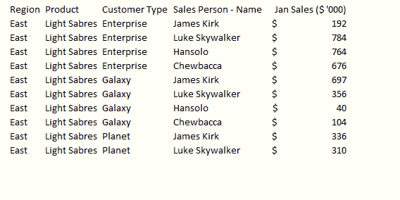
Excel Tables are an incredibly powerful way to handle a bunch of related data. Just select any cell with in the data and press CTRL+T and then Enter. And bingo, your data looks slick in no time. This has to be the best and easiest formatting tip.

Excel Formatting Tips - Use tables to format data quickly

Learn more about Excel Tables.

2. Change colors in a snap

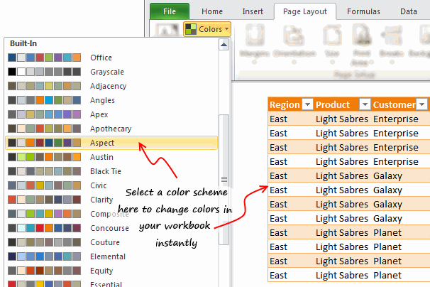
So you have made a spreadsheet model or dashboard. And you want to change colors to something fresh. Just go to Page Layout ribbon and choose a color scheme from Colors box on top left. Microsoft has defined some great color schemes. These are well contrasted and look great on your screen. You can also define your own color schemes (to match corporate style). What more, you can even define schemes for fonts or combine both and create a new theme.

Use color schemes to change formatting quickly - excel tip

3. Use cell styles

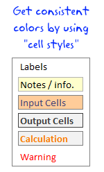
Consistency is an important aspect of formatting. By using cell styles, you can ensure that all similar information in your workbook is formatted in the same way. For example, you can color all input cells in orange color, all notes in light gray etc.

Apply consistent formatting with cell styles in Excel

To apply cell styles, just select all the cells you want to have same style and from Home ribbon, select the style you want (from styles area).

Learn how to use cell styles in Excel.

4. Use format painter

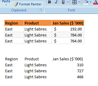
Format painter is a beautiful tool part of all Office programs. You can use this to copy formatting from one area to another. See below demo to understand how this works. You can locate format painter in the Home ribbon, top left.

Use format painter to format data quickly

5. Clear formats in a click

Sometimes, you just want to start with a clean slate. May be it is that colleague down the aisle who made an ugly mess of the quarterly budget spreadsheet. (Hey, its a good idea to tell him about Chandoo.org) So where would you start?

Clear formatting of a cell (or range) in a snap

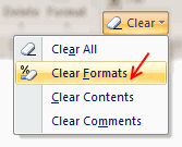
Simple, just select all the cells, and go to Home > Clear > Clear Formats. And you will have only values left, so that you can format everything the way you want.

6. Formatting keyboard shortcuts

Formatting is an everyday activity. We do it while writing an email, making a workbook, preparing a report, putting together a deck of slides or drawing something. Even as I am writing this post, I am formatting it. So knowing a couple of formatting shortcuts can improve your productivity. I use these almost every time I work in Excel.

  • CTRL + 1: Opens format dialog for anything you have selected (cells, charts, drawing shapes etc.)
  • CTRL + B, I, U: To Bold, Italicize or Underline any given text.
  • ALT+Enter: While editing a cell, you can use this to add a new line. If you want a new line as part of formula outcome, use CHAR(10), and make sure you have enabled word-wrap.
  • ALT+EST: Used to paste formats. Works like format painter (#4)
  • CTRL+T: Applies table formatting to current region of cells
  • CTRL+5: To strike thru.
  • F4: Repeat last action. For example, you could apply bold formatting to a cell, select another and hit F4 to do the same.

More: Formatting shortcuts for keyboard junkies

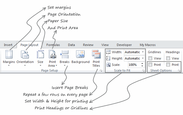
7. Formatting options for print

What looks great on your screen might look messed up, if you do not set correct print options. That is why, make sure that you know how to use these print settings. All of these can be accessed from Page Layout ribbon. For more, you can also use print preview and then “page settings” button.

Formatting options for printing

8. Do not go overboard

Formatting your workbook is much like garnishing your food. No amount of plating & garnishing is going to make your food taste good. I personally spend 80% of time making the spreadsheet and 20% of time formatting it. By learning how to use various formatting features in Excel & relying on productive ideas like tables, cell styles, format painter & keyboard shortcuts, you can save a lot of time. Time you can use to make better, more awesome spreadsheets.

10 Formatting Tricks only Excel experts would know

In addition to the above 8 formatting tips, I made a video explaining more tips. Watch it to learn 10 super cool, secret format tricks to take your spreadsheet game to next level.

  1. Merging without merging – centre across selection
  2. Merge multiple cells with “Merge across”
  3. No decimal points for large numbers with Custom cell formatting
  4. Showing numbers in Thousands or millions with Custom cell formatting
  5. New line in a cell with ALT+Enter
  6. Copy widths alone with paste special
  7. Skip zero in chart labels with custom cell formatting
  8. Align & distribute charts with alignment tools
  9. Show total hours with [h]:mm custom code
  10. Text format for very long numbers

What are your favorite Excel formatting tips?

Formatting (or making something look good) helps you get great first impression. I am always looking for ways to improve my formatting skills. While a great deal of formatting skill is art (and personal taste), there are several ground rules to follow as well. Applying ideas like consistency, alignment, simplicity and vibrancy goes a long way.

What formatting tips & ideas you follow? Please share them with us using comments.

Learn how to make better spreadsheets

Join Excel School & Make awesome Excel sheets

In my Excel School program, we focus not just on teaching Excel, but also teaching you how to make awesome Excel workbooks. You can see how I format my data, charts, dashboards & reports and learn hundreds of tips on formatting.

Even the lesson workbooks are beautifully formatted & packed with fresh ideas for you to try.

Consider joining our Excel School program, because you want to be awesome in Excel.

Facebook
Twitter
LinkedIn

Share this tip with your colleagues

Excel and Power BI tips - Chandoo.org Newsletter

Get FREE Excel + Power BI Tips

Simple, fun and useful emails, once per week.

Learn & be awesome.

Welcome to Chandoo.org

Thank you so much for visiting. My aim is to make you awesome in Excel & Power BI. I do this by sharing videos, tips, examples and downloads on this website. There are more than 1,000 pages with all things Excel, Power BI, Dashboards & VBA here. Go ahead and spend few minutes to be AWESOME.

Read my storyFREE Excel tips book

Overall I learned a lot and I thought you did a great job of explaining how to do things. This will definitely elevate my reporting in the future.
Rebekah S
Reporting Analyst
Excel formula list - 100+ examples and howto guide for you

From simple to complex, there is a formula for every occasion. Check out the list now.

Calendars, invoices, trackers and much more. All free, fun and fantastic.

Advanced Pivot Table tricks

Power Query, Data model, DAX, Filters, Slicers, Conditional formats and beautiful charts. It's all here.

Still on fence about Power BI? In this getting started guide, learn what is Power BI, how to get it and how to create your first report from scratch.

40 Responses to “Looking up when the data won’t co-operate (case study)”

  1. Sumit Bansal says:

    Nice Trick.. Clever use of cell references

    Here is a formula I tried to create:
    =SUMPRODUCT(((NOT(ISERROR(SEARCH(L5,B4:H14))))*1),(B5:H15))

    It takes care of Caveat #1 (can handle text), but Caveat #2 remains.

  2. PeterB says:

    In situations like this, I will often use VBA to restructure the data (2 columns: dates and values) on to a new worksheet. I can then use this 'clean' source for data analysis (formula or pivot table).

    =SUMPRODUCT(((NOT(ISERROR(SEARCH(L5,B4:H14))))*1),(B5:H15)) and complex formulae in general are all very well but when you come back to them in a few weeks / months time, it is not at all easy to see what they do and what the limitations are.

  3. Somendra Misra says:

    Hi Chandoo,

    I had used this type of cell ref. various times while calculating average.
    But for the situation here try below formula . Note this is an array formula and must be confirmed with Ctrl+Shift+Enter.

    =SMALL(IF(MMULT((L5=B4:H14)*IF(ISNUMBER(B5:H15),B5:H15),{1;1;1;1;1;1;1}),MMULT((L5=B4:H14)*IF(ISNUMBER(B5:H15),B5:H15),{1;1;1;1;1;1;1})),1)

    Regards,

  4. Somendra Misra says:

    Hi, I think Using SEARCH in here will create a problem say there is a text like SUN and another text SUNLIGHT both result will be added by SUMPRODUCT.

    Regards,

  5. Elias says:

    Array option.

    =SUM(IF(MOD(ROW(B4:B14),2)=MOD(ROW(B4),2),IF(B4:H14=L5,B5:H15)))

    Regards

    • Michael (Micky) Avidan says:

      @Elias,
      Nice approach.
      Although not requested - the formula I suggested closes all possibilities.
      Criteria: _____ Value to retrieve:
      Date__________ Numeric
      Date__________Textual
      Textual________Numeric
      Textual________Textual
      While your formula copes with only the 3 first combinations.
      Michael (Micky) Avidan
      “Microsoft® Answer” – Wiki author & Forums Moderator
      “Microsoft®” MVP – Excel (2009-2015)
      ISRAEL

      • Elias says:

        @Michael,

        Sorry but I don’t understand your point. I believe the challenge was to return the summary of a given date. What is your really volatile formula doing that mine is not?

        Regards

        • Michael (Micky) Avidan says:

          @Elias,
          I didn't say that the challenge differs from what you just mentioned/aimed to nor that your formula doesn't provide the requested result.
          Please read my previous comment again and focus on the last combination (TEXT / TEXT).
          I, myself, always try to provide a global Formula that is capable to handle all sorts of data.
          Michael (Micky) Avidan
          “Microsoft® Answer” – Wiki author & Forums Moderator
          “Microsoft®” MVP – Excel (2009-2015)
          ISRAEL

          • Elias says:

            @Michael,
            I see your point, but you are missing the below points if you are trying to cover all sorts of data.

            What happened if the lookup value does not exist?

            Do you want the first, second, summary, concatenation of the values if the look value is repeated?

            See they are too many possibilities to be cover with just one formula.

            Regards

  6. Michael (Micky) Avidan says:

    1) The range: B4:H15 was named: RNG.
    2) The following Array Formula was "retrieved from my sleeve" and I hope it can be shorten.
    3) The formula seems to take care of BOTH(!) caveats.
    -------------------------------------------------------------------------------
    =OFFSET(INDIRECT(ADDRESS(SMALL(IF(RNG=L5,ROW(RNG),""),1),MOD(SMALL(IF(RNG=L5,(ROW(RNG))+COLUMN(RNG)/10),1),1)*10)),1,)
    -------------------------------------------------------------------------------
    Michael (Micky) Avidan
    “Microsoft® Answer” – Wiki author & Forums Moderator
    “Microsoft®” MVP – Excel (2009-2015)
    ISRAEL

    • Elias says:

      @Michael,

      Check what happened with your result if you type 41927 in D5.

      Regards

      • Michael (Micky) Avidan says:

        Correct. Didn't predict that.
        Will find time to work something out.
        Michael (Micky) Avidan
        “Microsoft® Answer” – Wiki author & Forums Moderator
        “Microsoft®” MVP – Excel (2009-2015)
        ISRAEL

      • Michael (Micky) Avidan says:

        @Elias,
        Let's hope the following Array Formula "closes all open doors".
        Again - it has nothing to do with your formula which works fine as long as the 3 first mentioned combinations are concerned.
        -------------------------------------------------------------------------------
        =INDEX(RNG,LARGE(IF(RNG=L5,MOD(ROW(RNG)-1,2)*(ROW(RNG)),""),1)-2,(MOD(SMALL(IF(RNG=L5,(ROW(RNG))+COLUMN(RNG)/10),1),1)*10)-1)
        -------------------------------------------------------------------------------
        Michael (Micky) Avidan
        “Microsoft® Answer” – Wiki author & Forums Moderator
        “Microsoft®” MVP – Excel (2009-2015)
        ISRAEL

        • Elias says:

          Ok, if you insist. The following will cover all the scenarios you listed. However, I’ll never recommend/use such of formula.

          Defined names:
          rDat = $B$4:$H$15
          rRow =ROW(rDat)-MIN(ROW(rDat))+1
          rCol =COLUMN(rDat)-MIN(COLUMN(rDat))+1
          rInc =MOD(rRow,2)=MOD(MIN(rRow),2)

          L6=INDEX(rDat,MAX(IF(rInc,IF(rDat=L5,rRow)))+1,MAX(IF(rInc,IF(rDat=L5,rCol))))
          Array Enter

          Regards

        • Frank says:

          @Michael,

          unfortunately, your array formula still seems to return wrong results (eg 3-Nov).

  7. Magda says:

    If data are organized like in the example, ie. looks like a calendar, the INDEX formula seems quite simple:
    =INDEX($B$4:$H$15,ROUNDDOWN((L5-B4)/7,0)*2+2,MOD((L5-B4),7)+1)

    • Marc says:

      Yours is effectively the same as what I just came up with, and I believe this is the optimal answer to this particular problem.

      My solution, before I saw yours:
      =OFFSET(B5,QUOTIENT(L5-B4,7)*2,MOD(L5-B4,7))

      OFFSET will work for an arbitrary list size, but INDEX might be easier to read.
      QUOTIENT does the round and division in a single step.

  8. XOR LX says:

    If there's an improvement over Elias's solution then I for one can't see it.

    Perhaps a non-CSE version which would also mean that only two references (B4:H14 and B5:H15), as opposed to three (B4, B4:B14 and and B5:H15), would require manually amending should the data range change, i.e.:

    =SUMPRODUCT((ISEVEN(ROW(B4:H14)-MIN(ROW(B4:H14)))*(B4:H14=L5)*B5:H15))

    I suppose we could make it a single, uniform range reference:

    =SUMPRODUCT((ISEVEN(ROW(B4:H14)-MIN(ROW(B4:H14)))*(B4:H14=L5)*OFFSET(B4:H14,1,,,)))

    which might be more appropriate should we e.g. wish to use a Defined Name for our range, i.e.:

    =SUMPRODUCT((ISEVEN(ROW(Rng)-MIN(ROW(Rng)))*(Rng=L5)*OFFSET(Rng,1,,,)))

    though whether that compensates for the extra, volatile function call is something to be debated.

    Regards

  9. Mahir says:

    I have tried something and then my Excel workbooks got shut down. Maybe that was too much?

    Anyway here is what I've tried:

    =SUMPRODUCT(INDEX(B5:H15;IF(ISEVEN(ROW(B5:H15));ROW(B5:B15)-ROW(B5)+1);{1\2\3\4\5\6\7}))

    Guess that was wrong? Would this approach work anyway?

    Looking forward to learn something from you Excel Experts.

  10. XOR LX says:

    @Michael Avidan

    As it stands that is not a very rigorous construction.

    You say "I, myself, always try to provide a global Formula that is capable to handle all sorts of data", which is a wonderful philosophy, but isn't it at least as important that we ensure that our formulas are independent of the row and column references of the data range in question, so that, should that range change, we do not have to re-work our solution?

    What happens with your formula, for example, if RNG is instead re-located one row down, from B4:H15 to B5:H16?

    When a formula is reliant upon the addition/subtraction of certain constants within the formula, which themselves are necessarily dependent upon the specific rows/columns in which the data lies at any given time (e.g. the -1 in MOD(ROW(RNG)-1,2)), then that formula is not a very flexible one.

    Hence the reason for my choice of a slightly longer construction:

    ROW(B4:H14)-MIN(ROW(B4:H14))

    which ensures that this part of the calculation is not dependent upon the precise location of the data range within the worksheet, and so will give correct answers even if that range is re-located.

    Regards

  11. Haz says:

    {=OFFSET(B4,MAX((B4:H15=L5)*ISODD(ROW(1:12))*ROW(1:12)),MAX((B4:H15=L5)*ISODD(ROW(1:12))*COLUMN(A:G))-1)}

    • Haz says:

      Non-array formula:
      =INDEX(B4:H15,SUMPRODUCT((B4:H15=L5)*(ROW(B4:H15)-ROW(B4)+1)*ISODD(ROW(B4:H15)-ROW(B4)+1))+1,SUMPRODUCT((B4:H15=L5)*(COLUMN(B4:H15)-COLUMN(B4)+1)*ISODD(ROW(B4:H15)-ROW(B4)+1)))

      Using one range (B4:H15), one reference (B4), one lookup value (L5) and no INDIRECT or OFFSET.

  12. MF says:

    My trial with defined names:

    DateRange
    =$B$4:$H$4,$B$6:$H$6,$B$8:$H$8,$B$10:$H$10,$B$12:$H$12,$B$14:$H$14

    Position
    =RANK('lookup problem'!$L$5,DateRange,1)

    L6
    =OFFSET(B4,ROUNDUP(Position/7,0)*2- 1,IF(MOD(Position,7)=0,6,MOD(Position,7)-1))

  13. Jeff Weir says:

    I'd probably just run with something like:
    =SUMPRODUCT((B4:H14=L5)*(MOD(ROW(B4:H14),2)=MOD(ROW(B4),2))*B5:H15)
    ...which is basically the same as Elias' but without the IFs

  14. Bermir says:

    The opposite of elegant but it works...

    =INDEX(B4:H15,IFERROR(MATCH(L5,B4:B14,0),0)+IFERROR(MATCH(L5,C4:C14,0),0)+IFERROR(MATCH(L5,D4:D14,0),0)+IFERROR(MATCH(L5,E4:E14,0),0)+IFERROR(MATCH(L5,F4:F14,0),0)+IFERROR(MATCH(L5,G4:G14,0),0)+IFERROR(MATCH(L5,H4:H14,0),0)+1,IFERROR(MATCH(L5,B4:H4,0),0)+IFERROR(MATCH(L5,B6:H6,0),0)+IFERROR(MATCH(L5,B8:H8,0),0)+IFERROR(MATCH(L5,B10:H10,0),0)+IFERROR(MATCH(L5,B12:H12,0),0)+IFERROR(MATCH(L5,B14:H14,0),0))

    • Bermir says:

      =INDEX(B4:H15,
      IFERROR(MATCH(L5,B4:B14,0),0)+
      IFERROR(MATCH(L5,C4:C14,0),0)+
      IFERROR(MATCH(L5,D4:D14,0),0)+
      IFERROR(MATCH(L5,E4:E14,0),0)+
      IFERROR(MATCH(L5,F4:F14,0),0)+
      IFERROR(MATCH(L5,G4:G14,0),0)+
      IFERROR(MATCH(L5,H4:H14,0),0)+1,
      IFERROR(MATCH(L5,B4:H4,0),0)+
      IFERROR(MATCH(L5,B6:H6,0),0)+
      IFERROR(MATCH(L5,B8:H8,0),0)+
      IFERROR(MATCH(L5,B10:H10,0),0)+
      IFERROR(MATCH(L5,B12:H12,0),0)+
      IFERROR(MATCH(L5,B14:H14,0),0))

  15. HF says:

    Named Range
    rownum = SUMPRODUCT(('lookup problem'!$B$4:$H$14='lookup problem'!$L$5)*ROW('lookup problem'!$B$4:$H$14)*ISEVEN(ROW('lookup problem'!$B$4:$H$14)))

    Formula
    =OFFSET($A$1,rownum,MATCH(L5,INDIRECT("$B"&rownum&":$H"&rownum),0))

  16. Venky says:

    How about SUM(IF(B4:H14=L5,B5:H15)) with array..it should work

  17. xen says:

    Sorry, Chandoo, you can't find stuff this way in every possible scenario.
    What if 2014-10-01 sales would equal 41.927 ? Which is serial number for 2014-10-15 ? SUMIF would fail to retrive correct answer. And your example data suggest that such number is possible in your table.

    It's better not to search through dates and numbers at the same time.

    If I'd solve a problem like this, it'd reformat table first so I get one column with dates and the other with numbers.

    In this case, formula to form date column would be:
    =INDIRECT(ADDRESS((INT((ROW()-4)/COUNT($B$4:$H$4))+1)*2+2;MOD(ROW()-4;COUNT($B$4:$H$4))+2;4;1))
    and numbers would be the same formula with sight adjustment (+3 instead of +2 at the end of first argument):
    =INDIRECT(ADDRESS((INT((ROW()-4)/COUNT($B$4:$H$4))+1)*2+3;MOD(ROW()-4;COUNT($B$4:$H$4))+2;4;1))

    And now you got two columns that you can safely use for searching!

  18. xen says:

    Oops, sorry, you actually mentioned that it doesn't work if number=date! I missed that part 🙁

  19. Vad says:

    ={OFFSET(A1,SUM((B4:H14=L5)*ROW((B4:H14))),SUM((B4:H14=L5)*COLUMN((B4:H14)))-1)}

    Works for all data... the solution I got for indirect looks little lengthy

  20. Rajesh says:

    I want to count last 20 records of a person, whose marks is greater than 2 and grade "manager". ....

    Assume A1 has got names (James, John...etc...)
    A2 "Manager"

    A3 "2"

    Someone please reply

  21. Rajesh says:

    I want to count last 20 records of a person, whose marks is greater than "2" and grade "Manager"

    Assume A1 "geroge" A2 "Michael" A3 "George" etc...name can found anywhere in the rows

    B1 "Manager" B2" clerk"

    C1 "2" C2, "4"

    please reply

  22. Marc says:

    Simplest I can come up with. No limitations for either 1 or 2. This does assume dates are an ordered list with 7 per row, and 2 rows per set. Assuming this is always true this will work for an arbitrary long list of dates.

    =OFFSET(B5,QUOTIENT($L$5-$B$4,7)*2,MOD($L$5-$B$4,7))

    • Michael (Micky) Avidan says:

      @Marc,
      Nice approach - however, as there are no "Negative Dates" - try:
      =OFFSET(B5,INT(L5-B4)/7)*2,MOD(L5-B4,7))
      ——————————————————————————-
      Michael (Micky) Avidan
      “Microsoft® Answer” – Wiki author & Forums Moderator
      “Microsoft®” MVP – Excel (2009-2015)
      ISRAEL

  23. Vijaykumar Shetye says:

    =OFFSET(B4,ROUNDUP((L5-41911+1)/7,0)*2-1,MOD(L5-41911,7))

    B4 has been used as reference cell for OFFSET().

    FOR ROWS:
    ROUNDUP(....,0) gives the integer value of a division. In case of presence of a remainder, ROUNDUP will add 1 to the Quotient.
    As opposed to ROUNDUP(), the INT() or QUOTIENT() functions eliminate the remainder.

    41911 = 01-Sept-2014, the first date in the data.

    *2 has been used because there are 2 columns per set of data.

    /7 has been used because there are 7 columns per set of data.

    For columns
    MOD(L5-41911,7))

    Vijaykumar Shetye,
    Panaji, Goa, India

  24. Awais says:

    This is how i did it

    {=INDEX(B4:H15, MAX((L5=B4:H15)*ROW(B4:H15))-2, MAX((L5=B4:H15)*COLUMN(B4:H15))-1 )}

  25. Paul says:

    Here's my solution:

    =INDEX(B4:H15,MATCH(1,MMULT(--(B4:H15=L5),TRANSPOSE(COLUMN(B4:H15)^0)),0)+1,MATCH(1,MMULT(TRANSPOSE(--(B4:H15=L5)),ROW(B4:H15)^0),0))

Leave a Reply