Story of my first ever 200KM bike ride (plus an Excel dashboard with ride stats)

Share

Facebook
Twitter
LinkedIn

Ok people. Let me tell you that this post is almost not about Excel. It is about how one Excel blogger’s (yours truly) dream of long distance cycling came true. So sit back, grab your favorite drink and read between sips.

PS: if you just want to see the dashboard, click here.

So what is this all about?

Last Sunday (27th July) & Monday (28th), I finished my first ever 200KM bicycle ride. I rode for a little more than 12 hours, burned 5,179 calories & rode 206 kilometers.

It is definitely one of the most memorable, tiresome & uplifting experiences in my life. So naturally, I want to share the story with you.

Thats me at the end of 118 km ride on Day 1 - near Annavaram village entrance

Where it all began

Around late last year, I read a book called Free Country by George Mahood. It is a story of two young British lads cycling from Lands End to John O’ Groats (from one end of Britain to another) without spending a penny of their own money. While reading the book, I kept thinking, ‘I should do something mildly similar one day’.

But I did not do much cycling in the next several months. Until…,

I read truly inspiring story of how adc cycled from Manali to Leh (500 km). The story is special because the terrain between Manali & Leh is filled with high altitude passes, dangerous mountain roads, harsh weather, almost no habitat & breath taking scenery.

That travelogue motivated me enough to get out my dusty cycle from garage and start riding it.

Soon I was riding 20 KM per day. I started doing a few long rides (~40km) in the weekends to build strength.

Once I felt confident, I discussed my plans for a longer ride with Jo (my wife). She was a little apprehensive as I have never done something like that and long rides could mean increased chance for injury or accident.

Finally we agreed that doing a round trip to Annavaram (a small temple town 118 km away from our home) would be reasonable. The roads to Annavaram are in excellent condition. There is ample help available all the way (plenty of food stops, villages & towns along the way). Plus in case of fatigue or injury, I could easily hitch a ride back home.

I fixed on the dates 27 & 28th of July for ride. Weather app on Jo’s iPad said there is 70% chance of rain. I kept my plans fluid & wanted to ride only if there is no rain in the morning when I started.

Route Map

Here is the route I took (link).

Day 1 – Vizag to Annavaram (118 km, 7:34 hrs riding)

I woke up at 4:45 AM and unlocked the doors immediately to see if there is any rain. No rain and the skies looked ok. I got ready, had a glass of milk & woke up Jo. She gave me a farewell hug and I left the house at 5:24.

The initial 20 km was a breeze to ride. The route so far is familiar as I bicycle on it almost everyday.

After riding 25  km, I took a short water break.

State highway 38 looked pleasant & fresh in the morning

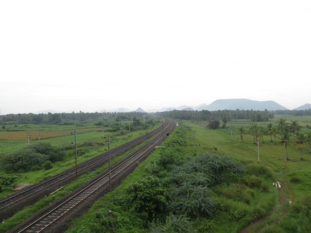
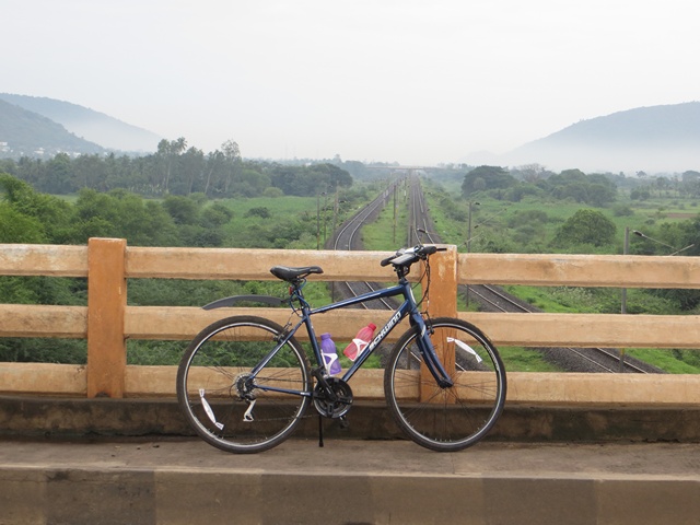
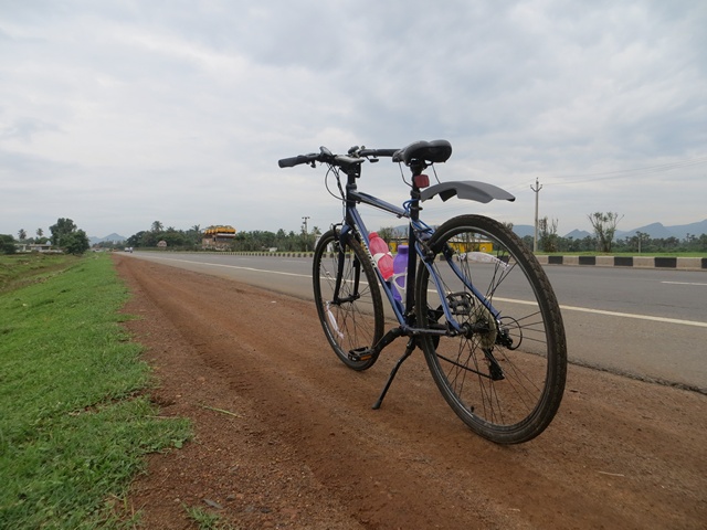
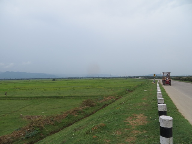
I barely rode for another 4 km and stopped again, this time to enjoy the view from top of a flyover. The rolling hills, green rice fields, railway track, chirping birds & fresh morning air provided perfect setting for a few pictures.

Rolling hills, green rice feilds, train track & beautiful sky, the route had it all

My ride - Schwinn Sporterra is all ready

Soon I left the state highway & joined national highway 45 (and 16 too). This is a 4 lane highway with wide shoulder. Unlike in US (and many other western countries), in India bicycles, pedestrians and many other forms of moving objects are allowed on highways. The best part of riding on national highway is that the gradients are better. Next 15 km felt like one long flat ride.

I crossed Anakapalli (a small town on the outskirts of Vizag) and stopped for breakfast at 41 KM mark. 1/3rd distance completed!

After feasting on Idly, Dosa & a tea (traditional breakfast in south India), I resumed the journey at 8:10 AM.

Still no rains. So I rode on.

At around 50 KM mark, stopped for a quick drink of water & electral (oral re-hydration solution made with essential salts & minerals).

At a water stop near 50km mark. The national highway 45 looked flat & inviting.

Around 60 km mark I started feeling a little thirsty and wanted to stop for some tea. Soon (after 6km) found a road side tea stall. My original plan is to ride until 80k mark and stop for lunch.

But seeing that I finished 66km by 9:56AM, I have decided to ride until Annavaram (my destination for the day) before lunch.

After the tea stop, I rode for another hour to reach Nakkapalli (a small village on the highway). There I saw a fruit juice stall. Immediately stopped to have a full glass of banana juice. The shop owner told me that Annavaram is another 36 km from there. It  started drizzling now. I am a little worried that it may rain heavily.

But my fears were unfounded. Soon the skies cleared and I was on a climb. After riding just another 10 km, I had to stop again to quench my thirst and relax a bit. As I was sitting by the road side, a mini truck stopped next to me. the truck driver was curious to know where I am heading & my story. After chatting for a while they left me.

A selfie at 90km mark. Happy with the progress made so far

At 95KM mark, I stopped again for a quick snack (snickers bar). Soon 2 kids on a cycle approached me. They are Siva & Siva Ganesh. Siva Ganesh (eldest one, studying 9th class) wanted to test ride my cycle. He was curious to know how the gears work. He took the cycle for a short spin and returned. They spend another 5 minutes with me asking several questions.

Picture taken by the Mr. Siva. You can see their cyle next to mine.

Once again I found myself on a steady climb. And then there are strong head winds. My speeds dropped to the range of 10-15kmph. After a lot of pedaling & sweat, I crossed Tuni at 12:30PM.
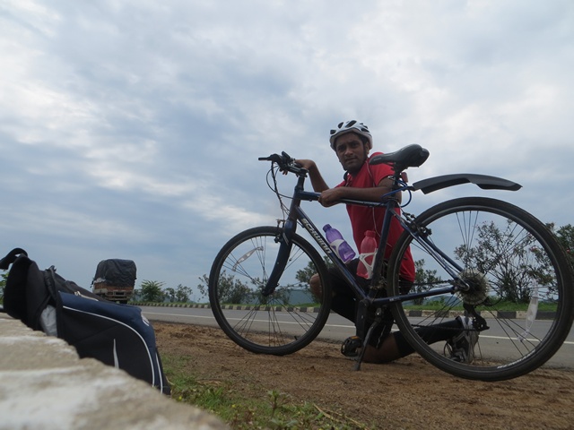
Selfie @ 100km mark

Selfie @ 100km Mark

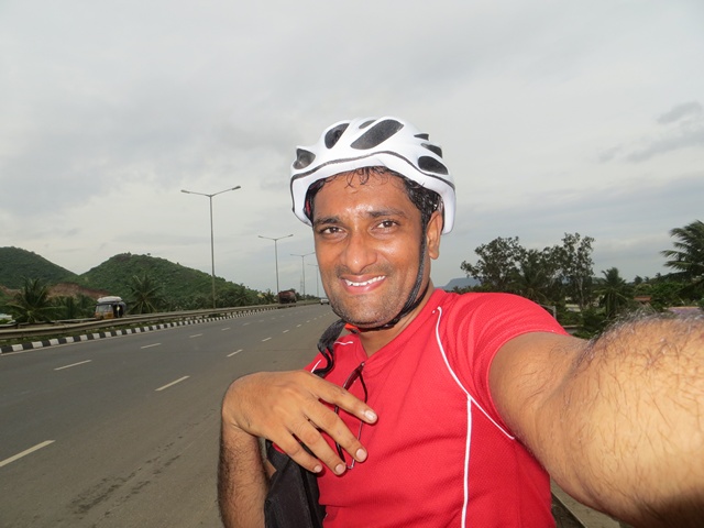
It took me another 30 minutes & 6 km of biking to reach a small temple village called Lova Gudi. By now my water bottles are emptied. So I stopped here to purchase a bottle of water. From here Annavaram (my destination) is 15 km. Normally I would have finished this distance in 40-50 mins. But after riding for 6 hrs, I find myself tired & sweaty. Plus the winds have picked up again. And to top it, almost all of this stretch is a climb.

I took a deep breath and resumed cycling.

The wind & gradient made my task all the more difficult. But I pressed on.

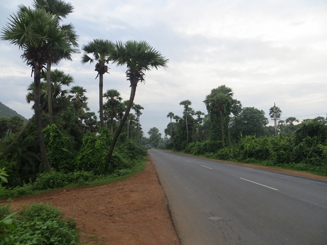
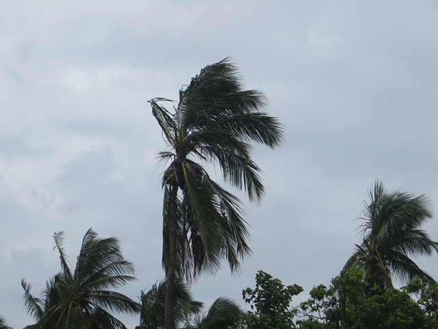
See how harsh the wind is. The coconut leaves are all bent.

Heavy head-winds made my climb even more difficult.

About 5 km away from Annavaram (around 110 km mark), someone in a car was waiting for me. As soon as he saw me, he waved his hands and stopped me. Turns out he is a biker from Vizag. He got curious upon seeing the site of a lone biker and wanted to know about me. We chatted for a while and exchanged phone numbers.

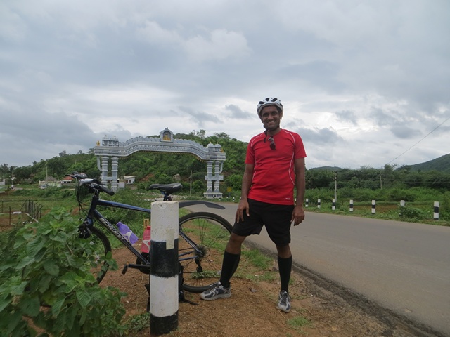
Finally at 2:50 PM, I reached Annavaram village gate. Yay!. It took me more than 9 hours & 30 minutes to reach here. Out of this riding time is 7:30 (it might have been slightly less than this as my tracking app – MapMyRide was not set to autopause for the first 65 km).

Finally, at Annavaram village gate after 9:30 hours of riding.

Thats me at the end of 118 km ride on Day 1 - near Annavaram village entrance

Day 1 – At Annavaram

I went to the first hotel I can find and ordered lunch. While waiting for lunch, I called Jo & my mom to tell that I reached safely.

After lunch I asked them if they have any rooms to stay. They have vacancies and I immediately took a room. I quickly showered and took a nap. But I could hardly sleep as my thighs and wrists were aching. It looked like I could not ride back and may have to take a bus to my home.

Originally I planned to visit the famous Annavaram temple in the evening. But my legs & back felt too sore to do anything. So instead I went for a short walk to explore the village in the evening.

Later I ordered dinner and watched some football on TV.

Around this time, I have decided to skip the return ride & take a bus instead. I told the same to Jo when I called her to say good night.

I kept waking up in the night due to one pain or other. I turned off the alarm at 6:15 AM and went back to sleep again.

Finally when I woke up at 8:00 I surprisingly felt rejuvenated and ready.

At that moment I decided to ride back home. My plan is to ride as far as I can and then take a bus.

Day 2 – Annavaram to Anakapalli (88 km, 4:30 hrs riding)

After a heavy breakfast & some coffee, I checked out of the hotel and started my return journey at 8:43 AM.

Since I have climbed & gained elevation yesterday, the first 40 km ride from Annavaram was almost downhill mixed with few flats. So I could maintain speeds between 20-30 kmph. At one point I even reached 43.5 kmph, although barely for a minute.

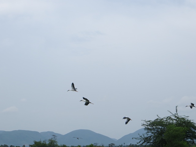
I did not stop anywhere for first 25 km. But then the views by the road are too breathtaking to ignore. So I stopped for a few pictures at 25k mark & again at 27k mark.

Selfie after 25km ride on Day 2

At the later stop, I found several open billed storks in the rice fields. It was a pleasure watching them forage for food & fly elegantly.

Open billed storks, flying away

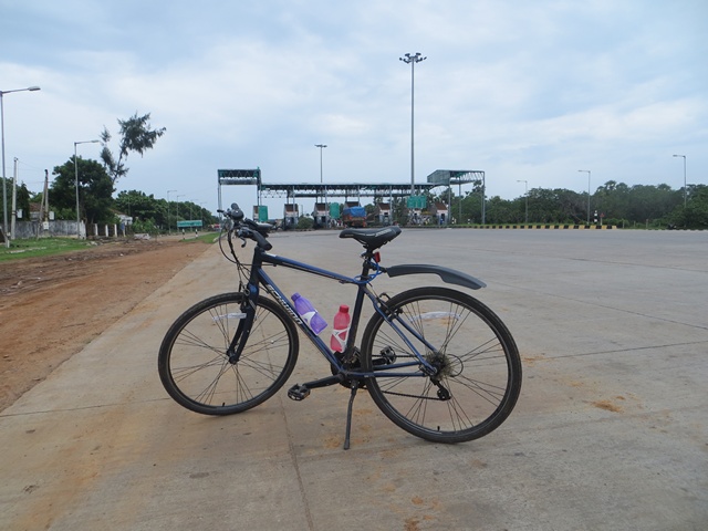
Pretty soon I reached the toll plaza. And yay!, no toll for me. Another reason to bike.

No toll for my bike, yay!

Had to stop again at 10:55AM to appreciate the beautiful green & blue views. Took a few pictures and resumed ride. Reached 50 KM by now.

Beautiful skies, green & blue views are inviting. So I took a break

At this point, I changed my plan to ride for 83 km. This will make the total distance as 200km.

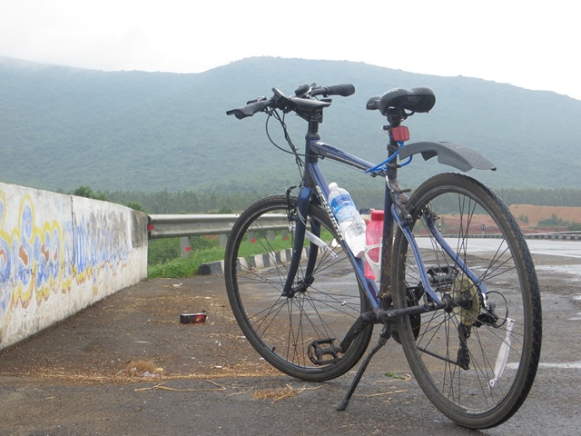
By 11:30, I reached Elamanchali (a small village 20 km away from Anakapalli, my destination for the day). By now it started raining quite a bit. My bike accumulated quite a bit of dirt & soot.

At 11:30 on day 2, the rains have started and my bike is all wet & dirty

By 1:00 PM, I reached outskirts of Anakapalli  and spotted a nice road side restaurant. Immediate stopped there for lunch. As soon as I stopped it started raining heavily. So I had a leisurely lunch spending close to an hour there. Finally the skies cleared at 2 PM and I resumed my ride.

When I was 3 km outside Anakapalli, a gentleman on motorcycle slowed down and rode with me for a few minutes. He asked me several questions about where I am riding, what I do, why I am riding etc. He even invited me to have lunch with him. But I had to decline as I already finished my lunch.

Finally, at 3:06 PM, I finished 88km and stopped my bicycle ride.

An empty mini truck going towards Sabbavaram (half way between where I stopped & my home) offered me a ride.

From Sabbavaram I took an Auto (a 3 wheeled taxi, also called as tuk-tuk) to my home.

And that marked the end of my first ever 200 km bike ride.

My impressions:

Growing up, I used to be the least fit kid in my school. I sucked at all sorts of sports. I got kicked out of football, hockey, badminton, cricket and all other sporting teams in school.

So naturally I assumed that I am not good for athletic activities.

Once I completed my studies and got a job, I realized the importance of living an active life. So I started jogging, cycling and playing sports.

Ever since I quit my job to start my own business, I became even more fitness conscious. Every year (since 2010), I have challenged myself to break personal barriers. When I first considered biking, I could not imaging anything beyond 50km per day. But with practice and motivation, I could finish this ride.

Few thoughts:

  • Do a few practice rides: I have been riding 20-30km per day for almost a month before taking up this challenge.
  • We underestimate our body: We can take on big challenges, endure pain & perform at our peak so much more than we estimate.
  • Drink & Eat well: I call my diet really healthy. We eat home cooked food 90% of the time. Most of our diet is veggies, fruits, milk, nuts, rice & wheat. Almost half of the vegetables & fruits we eat are grown in our back yard. We rarely drink and eat meat once a week.
  • Enjoy the ride: Stop and enjoy the scenery. Talk to fellow travelers and take ample breaks. Any distance can be covered easily.

Thanks to

  • Jo: for supporting & encouraging me.
  • My mom: for not freaking out when she learned about the ride.
  • Free Country & ADC: for the motivation
  • You: for supporting Chandoo.org so that I can chase my passions.

Now for an Excel Dashboard visualizing the ride

Soon after I got back, I started thinking about analyzing all the ride data. I did what I do best. I created an Excel dashboard to tell the 200km ride story.

Here is a snap shot of the dashboard (click to expand).

200km bike ride - visualized in an Excel dashboard

Click here to download the Excel Workbook.

It is unlocked. So go ahead and examine the file. Break it apart to understand the logic & formulas. Learn something new & be awesome.

How is this dashboard made?

Here I am going provide only the highlights. Please visit Excel Dashboards page for fantastic tutorials & explanations on how to make dashboards.

  • Tables: for structuring ride data. All the ride data came from MapMyRide. I used Doogal.co.uk to get elevation profile of the route.
  • Column & line charts: for the splits, speed & elevation.
  • Form controls: to make the charts dynamic & to control the Ride pics slideshow.
  • Picture links: to show one of the many ride pictures thru scroll bar form control.
  • Ample dose of formulas: Mainly INDEX, MATCH, SUMIFS & COUNTIFS.

More personal stories

If you are in the mood to know Chandoo.org & me a little more, check out these:

See you again with more awesome Excel stuff.

Facebook
Twitter
LinkedIn

Share this tip with your colleagues

Excel and Power BI tips - Chandoo.org Newsletter

Get FREE Excel + Power BI Tips

Simple, fun and useful emails, once per week.

Learn & be awesome.

Welcome to Chandoo.org

Thank you so much for visiting. My aim is to make you awesome in Excel & Power BI. I do this by sharing videos, tips, examples and downloads on this website. There are more than 1,000 pages with all things Excel, Power BI, Dashboards & VBA here. Go ahead and spend few minutes to be AWESOME.

Read my storyFREE Excel tips book

Overall I learned a lot and I thought you did a great job of explaining how to do things. This will definitely elevate my reporting in the future.
Rebekah S
Reporting Analyst
Excel formula list - 100+ examples and howto guide for you

From simple to complex, there is a formula for every occasion. Check out the list now.

Calendars, invoices, trackers and much more. All free, fun and fantastic.

Advanced Pivot Table tricks

Power Query, Data model, DAX, Filters, Slicers, Conditional formats and beautiful charts. It's all here.

Still on fence about Power BI? In this getting started guide, learn what is Power BI, how to get it and how to create your first report from scratch.

216 Responses to “Introduction to Excel SUMIFS Formula”

  1. cuboo says:

    Very useful, thank you!

  2. Jan Høgh says:

    Must... force.. IT-department... to UPGRADE THIS SORRY MESS TO Win7 & Office 2010!!!
    *drooooooool.....*

  3. Finnur says:

    I've been working with sumif formulas today and have been wondering how I can use 2 criterias or more. I have been reading about Dsum and Daverage. But, of course, this is much easier.

    So thanks!

  4. Ducheznee says:

    Of all the tips you've posted thus far, I can't think of one that will be more beneficial to me in my day-to-day. Wanting to include multiple criteria in my SUMIF formulas has long been a serious point of frustration.

    Question: How will this formula be handled by the conversion tool if someone opens my 2007 file with and earlier version of Excel?

    Thanks for sharing, Chandoo.

  5. bill says:

    I use these formulas a lot. I hope 2010 adds a bunch of additional ones. Don't forget that the criteria can be referenced in from cells outside the formula. This is really helpful for building a summary table. As an example of the versatility of the formula, using Chandoo's table, this formula =SUMIFS($C$2:$C$15,$A$2:$A$15,A2,$C$2:$C$15,F7) give a sum of 509 when the criteria value in A2 is "Pod Gun" and the criteria value in F7 is ">130". Also, wild cards can be used in the criteria formula... setting the "A2" cell reference to "*un" yields the same result.

  6. Chandoo says:

    @Ducheznee: Thank you. When you save a file with SUMIFS and open it in Excel 2003, the cells containing SUMIFS should show #NAME error (as the sumifs formula is not available in those versions). You can use one of the other methods (like SUMPRODUCT http://chandoo.org/wp/2009/11/10/excel-sumproduct-formula/ or SUM array formula http://chandoo.org/wp/2009/07/22/sumif-with-multiple-conditions/ ) to handle such cases.

    @Bill.. thanks 🙂

    @Jan Hogh: Totally agree with you. After using Office 2010 and Win 7, I dont feel like looking at windows xp comps.

    @Cuboo and Finnur: Thanks 🙂

  7. Eric Lind says:

    You know it's funny. When Excel 07 came out, I found I had to stop using SUMIFS because so many people were still using 03, but then you rescued me with SUMPRODUCT Chandoo! =)

  8. Abdul Kader says:

    Hi and 100 more
    as usual very impressive and cool especially with win7+office2010
    Many Thanks

  9. Fakhar says:

    What could be reason for not moving to Excel 2007+ as even large multinationals are also stuck with Excel 2003 when nobody has any doubt about their superiority over previous versions. So what might be the reasons behind this reluctance to adopt this much better product over an obsolete and less relevant in todays environment even by large multinationals?

    • Paul says:

      The larger the corporation the more applications are embedded and the easier it is to break things by up-editioning.  Induhviduals can fix broken logic however when you have 35,000 computers introduce errors jumping to the next version (no matter how great it is) ALWAYS get me reaching for the hoiday booking form!

  10. [...] The SUMIF swiss army knife April 26, 2010 at 5:42 PM | In General | Leave a Comment Tags: formulas, sumif, sumifs Chandoo wrote a very interesting explanation on how to use the SUMIFS function. [...]

  11. MPlee says:

    more and more i am using SUMIFS rather than VLOOKUP. it's invaluable when you want to supply multiple criteria in a table that has more than one or two dimensions. of course you have to make sure that each table entry is unique.

  12. Eric says:

    I am a teacher and need some help....how do I create a multiple sumif formula:

    I want to count/sum scores if they meet two criteria: Quiz and >=0

    If a student is Absent "A" I dont want it to affect their average. Any insight on an easy fix would be great. Thanks!

  13. [...] we know how to find sum of values that meet a criteria – we use either SUMIF, SUMIFS or SUMPRODUCT [...]

  14. Obisppo says:

    @ bill - you just saved me a TON of time! I hope I will pay it forward on your behalf. Thank you.

  15. gouse says:

    Hi, Iam preparing a salary bill of an employee for a period form July-2008 to June-2010. In this mean time he got promotion on 18-01-2009. From that day his salary hiked from Rs.10030 to Rs.10565. He got one increment on 18-01-2010. That day onwards his salary again enhanced from Rs. 10565 to Rs.11115. I prepared this bill in excel-2007 worksheet. I wish to split the salary in the months when he got hike in his salay, with excel formulas. But I am unable to do it. Can ypu help me please?

  16. Jawad Ahmed says:

    Being first time in chandoo.org i loved it sooooo much ... i become a great fan of chandoo cos its so simple and huge knowlege giving sites i have ever seen ..thanks a lot man ..god bless you

  17. Anish says:

    Hi Chandoo,
    I've been following Chandoo.org for some time now. Great work!
    Slight query regd. this post-
    I've used SUMIF\SUMIFS in the past, but I do have one grouse. The need for putting criteria in double quotes means I can't pull criteria from a cell reference which would make it much more powerful. i.e., instead of criteria ">150" how do i use criteria >$A$1 ? Some help please?
    Thanks, Anish

  18. Chandoo says:

    @Gouse.. you can use SUMIF or SUMIFS to sum all the salary amounts prior to promotion etc.

    @Jawad: Thank you 🙂

    @Anish: you can simply type >150 in A1 and then use that in formula like =sumifs(range, a1). If you cannot do that, you can use B1 to concatenate A1 with the operator you want.

  19. Anish says:

    Hey Chandoo,
    Thanks for that tip, Just tried it and it works! Nice!!
    Thanks again!.

    • Hirendra says:

      Anish, I am sure you did understand the side trick Mr. Chandoo showed you. But, a poor novice with this function like me, could not assimilate his trick. will you please be kind enough to show me in detail, or the actual formula you used? because, I am still fumbling with placing >150 in the formula!! Thanks a lot.

      • Hui... says:

        @Hirendra
        The format of Sumifs if
        =Sumifs(Sum Range, Criteria Range1, Criteria1, Criteria Range2, Criteria2 ...)
        =Sumifs(A1:A10, B1:B10, ">100")
        will sum A1:A10 where B1:B10 is > 100
        or
        =Sumifs(A1:A10, B1:B10, ">"&C1)
        will sum A1:A10 where B1:B10 is > C1

  20. kingmakeruday says:

    useful thank a lot but if u could more examples as a challenging i would be much better

  21. John Franco says:

    Hi Chandoo,

    Excellent review of the new SUMIFS function!

    Regarding the catch you mentioned above...

    If you want to send Excel files to users of previous versions you must convert SUMIFS. To make Excel 2003 users see results instead of an error the user must use SUMPRODUCT or Array formulas.

    This formula: =COUNTIFS('Sales'!$A$4:$A$400,"JAN",'Sales'!$V$4:$V$400,1)
    Turns into this one: =SUMPRODUCT(('Sales'!$A$4:$A$400="JAN")*('Sales'!$V$4:$V$400=1))

    This link may help:

    http://www.excel-spreadsheet-authors.com/sumif-multiple-7-ways.html/

  22. Tuttler says:

    I am trying to reuse the same criteria range but different criteria using SUMIFS; however, after establishing the first criteria range and entering the same for the second criteria range the result is zero. Is there a structure to reuse the same criteria range or include more than one criteria with the first criteria range? The data source structure is static but the values always change and I need to compare two data sources by sum.

  23. Chandoo says:

    @Tuttler... Can you give me an example of what you are trying to do. I am unable to visualize your problem.

  24. Tuttler says:

    The basic structure I tried using SUMIFS is: =SUMIFS(C:C,A:A,"Value A",A:A,"Value B",etc...). In order to get the result of using the same set of criteria_range, I used: =SUMIF(SUMIFS(C:C,A:A,"Value A"),SUMIFS(C:C,A:A,"Value B"),etc...)). Other criteria was used within each SUMIFS to further define the specific data set needed. Depending on the number of items required from the criteria_range the formula gets cumbersome.

  25. Ravi says:

    Hi Chandoo - great site! To follow up Tuttle's question, let say I wanted to determine podguns sales in the North AND the South.

    One way to try is maybe sumifs(podguns in the north) + sumifs(podguns in the south) although that might get cumbersome, I wonder if it might make more sense to try a dsum instead? I'm still in awe of / a little afraid of array functions {} but maybe you can use one as well?

    Ravi

  26. Harris says:

    Hi,

    Maybe you can help with a problem.
    I want to use sumifs to calculate sums based on 1 criteria being today's date.
    I am using the =Now() formula to automatically update the date. However, it is not summing. If i replace the =now() with a hardwritten date, it works.
    Any suggestions?

    Thanks,

  27. Hui... says:

    @Harris,
    try using =Today() instead of =Now()
    Today = Date
    Now = Date and Time

  28. Johnson Mathias says:

    Dear Chandoo

    Sumifs work great,
    but there is one short coming, one column one criteria

    I cannot get sum of two different months
    SUMIFS(Value,A19:A151,"April",A19:A151,"May")
    Sumifs gives a "0" when i put a second criteria
    I want to sum the sales of multiple/few months, the months are in Column A
    ie one column multi criteria
    Please Help

  29. Hui... says:

    @Johnson Mathias
    This is a short-coming in your logic not in Sumifs functionality
    .
    A cell in A19:A151 cannot be both April and May which is what you have asked Sumifs to do
    .
    Your query should be like
    =SUMIFS(Value Range,A19:A151,">"&DATE(2011,4,1),A19:A151,"<"&DATE(2011,5,30))
    .
    Give that a go

  30. Uzair says:

    why is that Sumif, sumifs, or sumproduct formulas not automatically update unless the source file is opened.

    They work fine same workbook but when external data source is involved it only work when source file is open.

    Please help help help!!!

  31. Hui... says:

    @Uzair
    There is a good article at Daily Dose of Excel on this which is worth a read
    http://www.dailydoseofexcel.com/archives/2004/12/01/indirect-and-closed-workbooks/
    .
    The comments also add other options
    .
    ps: There is no need to post here and in the Forums, they all get read

  32. [...] I then placed the same item indexes in data!A7:A46. This is all because I am lazy and I find the sumifs() formula a blessing: all I have to do now is to add up the results that correspond to (1) the chosen Product [...]

  33. Matias H says:

    Hui,

    I have a similar issue than 27), but I'm trying to have the criteria "Date" as a variable referred to in two separate cells. So I can define date ranges as I need.
    Sumifs gives a “0? when i put a the criteria
    Please help!

  34. Hui... says:

    @Matias H
    You can use something like
    =SUMIFS(B19:B151, A19:A151, ”>”&D1, A19:A151, ”<"&D2)
    Where D1 and D2 are the dates you want

  35. Matias H says:

    Thanks so much!!

  36. Cal C says:

    Using Excel 2007 I have changed and now almost exclusively use SUMIFS, its easier, and doing multiple criteria is quicker. I can track Date, Country, Dustributor and on and on easier with SUMIFS, that using SUMPRODUCT.

  37. meadrias says:

    Hi Chandroo (or whoever can help me! 🙂 )

    I need help - am very new to more advanced calculations in excel.
    My problem: I want to use 'sumifs', however the cells I want to add to the "sumrange" are not together (i.e.: c10+c6+c2+d2+e2) and want to include the conditions of sum only when c10 is not 0. I continue to get an error when I put this formula:
    SUMIFS(C10+C6+C2+C2+E2,C10,"0") and off course an error when I put the full formula I want which is something like this: SUMIFS(C10+SUMIFS(C6+C2+D2+E2,C6,"0"),C10,"0")

    Any help will be very much appreciated!

    EA

  38. Hui... says:

    @EA
    =IF(C10<>0,SUM(C2,E2,C6,C10),0)

  39. meadrias says:

    Thanks a lot Hui! 🙂

  40. AP says:

    I've reached the limits of my logic & after an hour of fiddling & researching have nothing to show for it.

    How do you select multiple criteria in a criteria range? Column A has sales person name, in some cases I need to sum together more than one sales person.

    When you enter the same range for both Criteria_range1 & 2 the result is 0. I've played with = combinations which works but is incorrect as Excel thinks I'm after a range.

    In effect what I want to do is:

    =SUMIFS(WEBI_LY,WEBI_BDM,"fosters group",WEBI_BDM,"sean crowe-maxwell",WEBI_BRAND,C3,WEBI_BUNDLE,D3)

    Many thanks in advance guys!

  41. Hui... says:

    @AP
    Your trying to do this:
    =SUMIFS(B2:B11,A2:A11,"a",A2:A11,"b")

    What that says is Sum Column B when Column A = "a" and Column A = "b"
    A single record can only be one or the other it can't be both
    .
    You need to use something like:
    =SUMIFS(B2:B11,A2:A11,"a")+SUMIFS(B2:B11,A2:A11,"b")
    .
    In your case
    =SUMIFS(WEBI_LY, WEBI_BDM, ”fosters group”, WEBI_BRAND, C3, WEBI_BUNDLE, D3) + SUMIFS(WEBI_LY, WEBI_BDM, ”sean crowe-maxwell”, WEBI_BRAND, C3, WEBI_BUNDLE, D3)

    • fred says:

      this exercise would be easily solved if Excell had an "or" function as in ”fosters group” or ”sean crowe-maxwell”. But assuming this is not the case, how do you solve this if instead of the above 2 conditions, there were 5, or 6? the function would indeed be long, tedious and prone to errors. In other words, what I'm really looking for (as well as other users I suppose) is a filter to be expressed as a function. Last but not least, very valuable posts.

      • Hui says:

        @Fred
        You can do this in one formula using Sumproduct
        =SUMPRODUCT(((A2:A11,”a”)+(A2:A11,”b”)),B2:B11)
        The + is effectively saying or
        so Where A2:A11 = a or b sum B2:B11

        • Tom says:

          Hi Hui,

          I have a similar issue and wanting to know if you can use SUMIF with Text Columns.

          Col A Col B Col C
          ProductName machineName Status
          MS Office Desktop1 In Use
          MS Office Desktop2 In Use
          MS Office Desktop3 Removed

          Want to sumifs for ProductNames installed on various machines with a particular status

          Tom

  42. AP says:

    @Hui | Thanks mate! Had that as my work around whilst awaiting a response here, was just hoping for something a little cleaner. All cool!

  43. g says:

    excellent-the example really helped

  44. Jackie says:

    Hi All,
    trying to resolve this, i need my criteria 1 to be equal either 4 or 5. The logic is correct, just not returning the results
    SUMIFS(E6:E108,C6:C108,AND(4,5),I6:I108,A122)

    Thanks in advance

  45. Hui... says:

    @Jackie
    I hate to disappoint but the logic is a little bit out
    What you have asked for is that a cell in Range C6:C108 has a value of 4 and 5, which a cell obviously can't have.
    And/Or aren't really suitable for use like this, although at first glance it does seem like they should be.
    .
    I'd recomend the following:
    =SUMIFS(E6:E108,C6:C108,4,,I6:I108,A122) + SUMIFS(E6:E108, C6:C108, 5, I6:I108, A122)

  46. Pete says:

    Hi, Is it possible to have the SUM_RANGE as a cell reference with the cell reference being a VLOOKUP formula result)?
    For example: data downloads from another program each month into sheet 1, with month 1 in (say) col D, month 2 in E etc. so it grows column wise each month. In sheet(2) is a table of 12 months with corresponding column references ( cell a1 has 001.2011 and cell b1 has "D:D" , a2 has 002.2011 and b2 has "E:E". In sheet 3 Z1 is a list ( being a1 to a12 dates. In Z2 is a Vlookup formula which looks up the relevant column reference (ie list choice 002.2011 gives "E:E" in Z2. In cell Z8 is the sumif formula : =SUMIF($A:$A,"wotnots",Z2). This should look at col A for wotnots and choose col E (month2).
    The cell accepts the formula but doesnt give a numerical result. Iam wanting to be able to change sumif parameter using list choice.

  47. Philip says:

    Hi,

    This related to Excel 2007. I have a sheet with multiple columns. Column B has dates (dd-mm-yyyyy) ranging from 1st to 31st of the month depending on the month. Column H has the amounts I want to sum when they are greater than zero. Each date can have multiple rows so the totals row is dynamic but the column rows are generally static.

    I want to sumif on the Column B values (day less than 25th) and Column H, as indicated, for values greater than zero.

    So far, my formula which sits a few rows below the total in Column H is not working:

    =SUMIF(B6:B164;VALUE(LEFT(TEXT(CELL("contents");"TT MMM JJJJ");2))"<25";H6:H164)

    I've stripped it back but the quotes seem to be giving me headaches? Any ideas?

    Kind regards,
    Philip

  48. ravi says:

    does it have to be a sumif? how about a sum with ifs and curly brackets?

    =SUM(IF(TEXT($b$6:$b$64,"dd")*10,$h$6:$h$164))))

    then hit ctrl shift enter for the array curly brackets?

    Ravi

  49. Johnson says:

    Hi Philip

    Regarding post 44) Philip November 21, 2011
    Your table seems to be A6:H164
    Try
    =SUMIFS($H$6:$H$164,$B$6:$B$164,"0")

    Works like a charm

  50. Johnson says:

    part of formula above is getting edited as HTML

    SUMIFS($H$6:$H$164,$B$6:$B$164,"=25-11-2011",$H$6:$H$164,"=0")

    Change the = signs with greater than & less than Signs

  51. Philip says:

    Dear Ravi and Johnson,

    Many thanks for your responses. Uhnfortunately, I've been too busy to try them out but as soon as I do, I'll let you know. @Ravi: I don't see where your formula is checking that the B column value is less than 25? Whether it is a SUMIF is for me secondary. It just has to before the logic I explained. Note that as I explained the 164 value is dynamic (in my fomula I actually use the "row()- 1" instead of 164. I just put the 164 to reduce the number of brackets.
    @Johnston: only the 25 (day) is static, the month and the year change.

  52. abdullah says:

    how i can do sumif function in excel with tow condition in the same criteria, for example: sumifs of any rang with condition 4=< X <=6 .
    thank you.

  53. Johnson says:

    Hey Philip
    I did not realize the day is static 25
    One solution would be to add a Say "J" column called "Day" =day(B1)
    Thus you get a usable day criteria

    SUMIFS($H$6:$H$164,$J$6:$J$164,”=25?,$H$6:$H$164,”=0?)

    Change the = signs with greater than & less than Signs

    I hope this helps

  54. FG says:

    To those wondering how to use an operand with a cell reference (and to the extent it wasn't already posted) you simply concatenate the operand in quotes with the cell reference using an ampersand. So if your condition is less than or equal to the contents of C5, you type:

    "<="&C5

  55. FG says:

    Hui, you seem to recommend summing the result of two SUMIFS with slightly different criteria to satisfy the need for what is essentially an OR() function. Can you use an AND() or an OR() as a condition, or is yoru solution the only way to accomplish that?

  56. FG says:

    My third and final post today: I answered my own question using Hui's comments above. To satisfy an OR condition (such as numbers between two values) you just repeat the range to be evaluated twice, once with a ">=" condition and once with a "<=" condition.

    Also, gotta give the obligatory shoutout...Chandoo's great!

  57. Misty says:

    Is it possible to use a cell reference in the range and sumrange in a sumif? I would like to type the sheet I want to reference in a specific cell and have the sumif formula reference that cell for the sheet information.

  58. FG says:

    Misty, I use sumifs whose source data is on a different sheet all the time, I've also done it across workbooks. I'm not sure what you're using the spare cell for as a reference though. Can you give an example of what you're doing? I don't want to give an overly wordy and unhelpful reply.

  59. Vineet says:

    Hi Chandoo!
    I have a problem....I have an Excel 2007 Sheet with Name of Dealers in Rows and Month wis Sales in Columns (Apr.10, Apr.11, May.10,May.11....Mar.11,Mar.12). I have a Dashboard Sheet where the user enters the starting month & ending month for e.g. Apr.11 TO Sep.11.
    I want to calculate the No of Dealers having registered some sales in the period i.e. Apr.11+May.11+.....Sep.11 should not be Zero. This needs to be calculated dynamically depending on the value entered in the Dashboard Month Field.

  60. Rick says:

    Hi Chandoo
    Great explanation of SUMIFS. But for summing up the values where data are spanning across multiple columns (e.g., data in 23 columns D:Z), is there a simple way? One could always write the SUMIFS statements for each column, using multiple criteria (e.g., criteria in 3 columns A:C), and then combine the results through simple addition, but this is not very elegant and in this case would require addition of 23 terms rather than one.
    For example, this sums one column (and could be repeated, tediously):
    =SUMIFS(D2:D10,A2:A10,A1,B2:B10,B1,C2:C10,C1)
    but this returns and error, rather than summing 23 columns:
    =SUMIFS(D2:Z10,A2:A10,A1,B2:B10,B1,C2:C10,C1)

    Thanks for your input and help.

  61. Rick says:

    Sorry, but I had mistyped my email address a minute ago (linked to my question on using SUMIFS across multiple columns). This time it is correct.

  62. Alec Berg says:

    Wow, great time saver. Thank you. I used it for the wildcard with the sumif.

  63. Lawrence says:

    Normal
    0

    false
    false
    false

    EN-US
    X-NONE
    X-NONE

    /* Style Definitions */
    table.MsoNormalTable
    {mso-style-name:"Table Normal";
    mso-tstyle-rowband-size:0;
    mso-tstyle-colband-size:0;
    mso-style-noshow:yes;
    mso-style-priority:99;
    mso-style-parent:"";
    mso-padding-alt:0in 5.4pt 0in 5.4pt;
    mso-para-margin:0in;
    mso-para-margin-bottom:.0001pt;
    mso-pagination:widow-orphan;
    font-size:11.0pt;
    font-family:"Calibri","sans-serif";
    mso-ascii-font-family:Calibri;
    mso-ascii-theme-font:minor-latin;
    mso-hansi-font-family:Calibri;
    mso-hansi-theme-font:minor-latin;
    mso-bidi-font-family:"Times New Roman";
    mso-bidi-theme-font:minor-bidi;}

     
    Is there any way to get SUMIFS to do either/or criteria?
     
    I was only able to get it to work with an array constant:
     
          =SUM(SUMIFS(sum_range,criteria_range1,criteria1,criteria_range2,{"A","B","C"}))
     
     
    However, arrays constants can’t use references like F1,F2,F3.


    Is the ONLY alternative to use SUMPRODUCT (much slower) or to use multiple SUMIFS (very long formula and high maintence).


    Lawrence
     

  64. Lawrence says:

    Yikes...what happened to my post?
    How do I edit out all that code???
    ~L
     

  65. Maria says:

    Thanks,  if everything was explained like this, everything would be easier to understand and do.

  66. andreaswpv says:

    works just great, but  I need to add an ampersand & to it to concatenate:

     =SUMIFS($D$2:$D$15,$B$2:$B$15,"bli",$C$2:$C$15,">"&50)

    Without the ampersand does not work at all with = or > or >=, just with a number. No matter if I put that in single or double or without marks. But with & works nicely. Sure I will use the sumifs quite some times.

  67. Hui... says:

    So that would make Sumproduct the
    Swiss Army Knife
    of Swiss Army Knives

  68. manoj Mishra says:

    give some more range.

  69. Richard Galicia says:

    I do stuffs like this in MS Excel 2003 by using the sumif  + concatenate function. Where concatenate resides in new column. =sumif($A$14:$A$27,"Pod GunEast",$C$14:$C$27) where Column A is concatenation (&) of Column B and C.

  70. Alghie says:

    Its very Helpful!! thank you

  71. Leo says:

    Hey Chandoo, you are really awesome!! Now I will use sumifs instead of sumproduct!

    Thanks a million!!

  72. Brianna says:

    Hello There. I found your blog the usage of msn.
    This is a very neatly written article. I'll be sure to bookmark it and return to learn more of your helpful information. Thanks for the post. I will certainly return.

  73. Vivek Singh says:

    Thanks Chandoo. It was very useful. No need to make a Pivot.

  74. JustiinCBU says:

    Is there any reason why a sumif statement will not work on a text cell with a < or > symbol in it?  I'm using these symbols to put data into buckets: >12 weeks, >26 weeks.  

    Cell A1: >12 weeks

    =SUMIFS(Value to Sum,criteria range,A1)
    =0
     
    Am I stuck with changing all the text to ranges: 12-25 weeks, 26-52 weeks? 

  75. anil says:

    dear sir,
    plz help formula us to 2003
    sumifs   in summary sheet

    me formula is
    sumifs('sheet 3 (cell s:s(value),'cell e:e(div),'summary sheet1 (cell c5 (ctv),'(sheet3(cell aa(status),summary sheet1 (cell c8 (applied),'(sheet3(cell k(month),summary sheet1 (old)

  76. Rajinder Singh says:

    Thanks Chandoo
    Your excel tips r really awsome & making us awsome.
    Can anyone help me out in this following condition:-
    Suppose I want to make different sales sheets each of Pod Gun, Blow Torch & Spit Bomb. Is it possible that as I type the entry in general table (containing all products), the entry also goes to its respective excel sheet ?
    Would b thankful

  77. Ella says:

    What if you want one of the criterias to pull from whatever is in a particular cell to the left?
    Right now my last criteria is unique customer names that I have to type, but I would rather the last criteria be a cell reference so that I can just drag the formula down.

  78. FG says:

    Hey Ella, see my posts above for using cell references and creating or conditions.  I pasted one of them below:
    "To those wondering how to use an operand with a cell reference (and to the extent it wasn’t already posted) you simply concatenate the operand in quotes with the cell reference using an ampersand. So if your condition is less than or equal to the contents of C5, you type:
    “<="&C5 "

  79. we can also use sumproduct same a sumifs right????

  80. Waqas Saeed says:

    Dear Chandoo,
    I don't have my own business neither appointed at a prominent position, despite of these shortcomings i've designated as "CEO" in the organization i'm employed at, and i acknowledge that its just b'caz of people like you. I'm fortunate to have you.
    CEO = Chief Excel Officer
    Wish you all the best!
    Thanks.


  81. Waqas Saeed says:

    Dear Chandoo,

    I don’t have my own business neither appointed at a prominent position, despite of these shortcomings i’ve designated as “CEO” in the organization i’m employed at, and i acknowledge that its just b’caz of people like you. I’m fortunate to have you.

    CEO = Chief Excel Officer
    Wish you all the best!
    Thanks.
     

  82. Ramesh says:

    It is really very good and helpfull!!!
    Great Chandoo.... 🙂

  83. Rebecca says:

    Question for you Chandoo, and maybe it is already addressed somewhere in the dialogue above. 
    Can the "SUMIFS()" formula fully replace the ARRAY formula that looks up criteria in multidimensional ranges? For example, I have the table below, I would like to search by Dept, Employee, Type, and then horizontal for a specific month. I cannot get the horizontal sum-if function to work.
     
    The following formulas return #VALUE!, but of course works when I change the sumrange to equal a specific month column.
    =SUMIFS($D$2:$F$5,$A$2:$A$5,"Sales",$B$2:$B$5,"Mary",$C$2:$C$5,"Contract",$D$1:$F$1,"MAR")

     
    A
    B
    C
    D
    E
    F

    1
    Dept
    Employee
    Type
    JAN
    FEB
    MAR

    2
    Finance
    John
    Contract
    160
    160
    160

    3
    Sales
    Bob
    Full-time
    195
    180
    185

    4
    Sales
    Mary
    Contract
    155
    150
    170

    5
    Sales
    Fred
    Full-time
    165
    155
    150

     
    I'd like to replace the cumbersome ARRAY formulas in my worksheets now that I have 2010, but the new SUMIFS formulas still seems to be limited in comparison (although it is much easier to understand).

  84. Peter says:

    Hey, great article and illustrations.
    This YouTube video is also good to see the sum, sum if and sum ifs functions in action - youtu.be/pYdOukeuENQ?a

  85. James Perry says:

    Sir....Brilliant tutorial with illustrations....and u r SuperBrilliant.
    Its a pleasure to watch ur vids.
    Blessing$.

  86. CA.Hitesh Bansal says:

    Great use of * i learnt today

  87. Edd says:

    Hi,
    Im having a problem with my SUMIFS formula. At the moment my formula looks like this =SUMIFS('Booked '!$H:$H,'Booked '!$F:$F,">="&$C$4,'Booked '!$F:$F,"<="&$D$4,'Booked '!$A:$A,$A8) This is looking up cancellation values within a certain date for a specifc sales person and is working fine. I now need to to add a criteria which will be the cancellation reason (the value of a specific cancellation reason) but i cannot figure out how to do this? everything keeps on coming back with a value of 0?
    Please help???

  88. Hui... says:

    @Edd

    Simply add another range and criteria
    eg: =SUMIFS(‘Booked ‘!$H:$H,’Booked ‘!$F:$F,”>=”&$C$4,’Booked ‘!$F:$F,”<="&$D$4,'Booked '!$A:$A,$A8, New_Range, New_Range Criteria )

    Note that the Range must be the same length as the previous ranges

    Posting a sample of the new formula and it';s criteria will assist us to help you further

    • Edd says:

      Thanks for that but im still getting a value of 0. I am looking up data on the same summary sheet but from a different tab so this is what my formula looks like when it works =SUMIFS(Cancelled!$H:$H,Cancelled!$F:$F,">="&$C$4,Cancelled!$F:$F,"="&$C$4,Cancelled!$F:$F,"<="&$D$4,Cancelled!$A:$A,$A8,Cancelled!J:J,E7) it comes back 0. What am i missing?

      Thanks sooo much for your help!!!

    • Edd says:

      @Hui

      Sorry that didnt copy correctly,

      Forumla that works =SUMIFS(Cancelled!$H:$H,Cancelled!$F:$F,">="&$C$4,Cancelled!$F:$F,"="&$C$4,Cancelled!$F:$F,"<="&$D$4,Cancelled!$A:$A,$A8,Cancelled!J:J,E7)

  89. Priti Bihani says:

    Hi Chandoo,

    I had a query regarding the SUMIFS formula...while defining the criteria for a given range, can i type the criteria in the formula instead of giving cell reference? I tried putting the criteria in quotes (tried both 'X' and ''X''...but excel is showing error in formula...Could u pls help me on this?

  90. […] Using SUMIFS formula (same tricks apply to AVERAGEIF, AVERAGEIFS too) […]

  91. Mary Tay says:

    hi,

    I just started to learning sumifs which is a great tool to use. I have a problem here and I need help.

    My data consists of salary and benefits details for professional staff, support staff, NBD staff & Management staff for both Singapore & Australia. I need to split total cost between:

    1. professional staff / Singapore - I got the answer for this since there's only 1 criteria
    2. Support/NDB/Mgmt staff / Singapore - i got a nil answer when I did this....
    SUMIFS('Cost report I'!AH3:AH43,'Cost report I'!C3:C43,'Cost summary'!A4,'Cost report I'!D3:D43,"Supp", 'Cost report I'!D2:D42, "NBD")

    I got the total cost for support staff but when i tried to add NBD....it gives me nothing. Can anyone enlighten me please.

    thanks

  92. Mary Tay says:

    thank you for your quick reply Hui. I just corrected the space but it is still not picking up the total cost.

  93. Lyman says:

    I have been using the SUMIFS formula to build a payroll Sheet for our office, however I track the hours in one sheet along with the days of the week and the specific job numbers, I then have another sheet that has all of the relevant employee information such as employee number and craft code, finally, I merge all of these onto a landing page where I am using combination VLOOKUP Formulas to auto-fill the needed information and then use dates and the top of the sheet in order to tell which week I am getting the information for. Now the SUMIFS are used in the hours columns to total all of the hours that the employee worked on the above date, and the specific job #, however as new employees come on and I add them to the list, it is no longer in alphabetical order, so when I use the filter buttons that are atop my sheet, It re sorts alphabetically but the formulas mess up and start referencing their old location even when they are unlocked or locked? Help Please?

  94. mrrk says:

    I do not remember clearly when it was the first time when I came across Chandoo's excel tips site - maybe in 2009, and thanks to the visuals and enjoyable diction, I am sure I will always remember the name Chandoo and will be able to come back to find the awesome solutions to my excel questions.

    Thank you, Chandoo! 🙂

  95. […] dashboard uses generous amounts of SUMIFS, COUNTIFS, INDEX, MATCH and VLOOKUP with an occasional […]

  96. […] Sumifs()  a close relation to Countifs() […]

  97. […] Sumifs()  a close relation to Countifs() […]

  98. […] least 5 cups of coffee, 2 hours of thinking, several hours of SQL, VBA, Pivot & SUMIFS, an hour of formatting & conditional formatting and may be 10 minutes on […]

  99. […] ???????? ???? ?????? (?? ?????????? ?????) […]

  100. Preethi says:

    Question: In the illustration above, how do i write a formula if i need the number of Pod guns & spit bombs sold in the North??
    Is it possible to find out the number of both Pod guns & Spit bombs sold in the same formula?

  101. abinaya says:

    Hi Chandoo,

    Couple of days back I got to know abt ur website thro a link. Amazing place to learn excel. found it realy help full. I have a question the in the sumifs formulae above, I want to find out the "Split Bomb" total for Both "North" and "West" region how do I find. I used the same sumif formulae with a {} to inuput North & West but its not working. Can u please help me

  102. sree says:

    very nice tips ....
    I like it

    I learn some thing from it

  103. pat poindexter says:

    i dont know how to use the downloaded excel workbooks that when downloaded are in xml format. Can you please tell me how to open them?

  104. Ben Cannon says:

    hi,
    i am using SUMIFS to reference to a seperate workbook (a timesheet)
    the formula figures out how many hours (entered) people did within specific date ranges. (creating a large consolodation spreadsheet).
    the problem is, when trying to update the references, all i see is #VALUE! unless i open up that specific sheet it is trying to reference to.
    is there a way for this formula to auto update? i read somewhere it needed =sum(ifs(------------)) but this doesn't work for me.

    any help is appreciated!

  105. Michael B says:

    I, have this problem: I need to find a function for each row of the data D2: I17. If the condition A2 = 1 + mount & year = equal; sumproduct (all 1 of range D2: I17). col B Col C and unique data . Thank you.

    A B C D E F G H I
    CRIT Mounth Year v1 v2 v3 v4 v5 v6
    1 January 2015 6 15 12 9 5 2
    2 January 2015 10 4 7 15 14 13
    3 February 2015 7 16 6 15 12 13
    4 February 2015 6 11 11 12 12 2
    5 March 2014 5 5 15 15 8 4
    6 March 2014 1 6 8 6 16 6
    7 April 2014 1 13 1 9 4 2
    8 April 2014 3 2 9 15 14 2
    9 May 2014 1 15 9 5 2 4
    10 June 2013 3 14 11 4 13 11
    11 July 2013 6 3 3 11 8 13
    12 August 2014 16 1 8 15 11 10
    13 September 2012 12 15 2 15 10 9
    14 October 2012 8 7 2 14 5 9
    15 November 2011 3 3 5 5 11 4
    16 December 2011 3 3 10 8 8 4

    • Chandoo says:

      Hi Michael,

      Thanks for your question. I am not sure I understand this. Can you explain better? May be tell us what is the answer you are expecting for first row?

  106. Chris McG says:

    In Lotus 1-2-3, you can enter criteria into database functions and avoid the primitive criteria range that Excel still requires (last used in Lotus 3.0). I cannot fathom why Microsoft Excel developers haven't changed the database functions so that they have this capability. I wonder if there is a way to communicate with them and express displeasure about the need for criteria ranges.

  107. thania says:

    Chandoo you are the best!!!!

  108. Charlene says:

    Thank you so much, it really helpful!!!

  109. Anindya Mukherjee says:

    THANKS FOR IT.IT'S VERY USEFUL.

  110. Magdy says:

    dear Sir.
    I need you help , sorry I know my English is not good , so I have Main table it' included Product and model . I need to make new table but product and Model not repeated together (look like primary key).
    thank for you cooperation

    Product Model
    jeans Levis
    jeans Levis
    jeans GAP
    jeans GAP
    T shirt Levis
    T shirt Buma
    T shirt Gap
    jeans Buma
    jeans Gap
    T shirt Buma
    jeans GAP
    jeans Levis
    T shirt Levis

    Product Model
    jeans Levis
    jeans GAP
    T shirt Levis
    T shirt Buma
    T shirt Gap
    jeans Buma

    • Hui... says:

      @Magdy
      Select A1:B14
      Then apply an Advanced Filter to the list
      And extract Unique Entries to a different location without any filtering

  111. Akash gulati says:

    HI TO CALCULATE THE SUM BETWEEN TWO RANGES.
    That Is suM ALL BETWEEN 1000-5000
    & 5000-10000.
    The formula i am applying is Sumifs(B3:B990,"1000")

    • Hui... says:

      @Akash
      =Sumifs(B3:B990,"gt1000",B3:B990,"lt5000")

      =Sumifs(B3:B990,"gt5000",B3:B990,"lt10000")

      swap gt and lt for Greater than and less than characters

  112. Jaishankar Soni says:

    Very nice article. Thank you very much.......

  113. Armand says:

    Not sure if possible but I need to do a sumif for a headcount by region and department. The regions will be listed vertically on column A3:A15 while the departments will be listed horizontally A2:G2.

    The issue is the departments are rollups with multiple departments falling into each rollup. Can I do a vlookup on the department to see which rollup it falls under and place that vlookup in a sumif?

    I hope I am asking that clearly.

  114. Sue says:

    I am trying this out exactly as above (SUMIFS) in Excel 2010 and it is returning a '0'. Any thoughts? Pretty sure its user error.. 🙂

  115. I am a liar says:

    Man!!!!
    you are my bro!!!

    I work on servers and use excel only to vlookup and stuff. I told in an interview that I am an advanced excel user as job was related to hardcore data. I got the job and now I am learning the "advanced excel"

    this was helpful

    Thanks
    🙂

  116. Fazil Ahamed says:

    Hi,

    Good day!

    Hope to be well.

    I hereby inform to that, I was working as an assistant accountant, will need to Excel skills from basic to advance level now, so kindly provide me tremendous advice for how to improve those kind of Excel skills by myself.

    Looking forward to your prompting response

    Regards & Thanks

  117. Shubam Karnal says:

    These are very helpful and make work easier. Thanks a lot for sharing the knowledge Chandoo.

    Thanks & Regards
    Shubam

  118. Dilip says:

    I m big fan to chandoo.org b'coz chandoo logic is too simpla and work

  119. TJ says:

    This just saved me hours of work - thank you! You have a new fan!

  120. shabarish says:

    Awesome. So useful. Thank you so much.

  121. Blackbeard says:

    I am having a problem writing index formulas, I have a colum of names in A and a colum of numbers in F In another cell in E2 I want to input a number and get the closest 3 values put in 3 new cells with their corresponding names from the details in colum A.

    Thanks for any help you can give,
    All The Best

  122. i venkat rao says:

    i owe you alot to this site to giving me chance to learn wonderfull formulas in excell

  123. Tushar says:

    thank you....

  124. Usman says:

    Hi Chandoo,

    how would you determine the "Sales of Pod Gun AND Blow Torch in North" using SUMIFS?

    It seems like if we use multiple conditions from same column, it doesnt execute the right number, instead gives a 0!

  125. ROHIT SHARMA says:

    Hi,
    I would like to make the productivity sheet with the use of SUMIFS function in excel, so please give a advice to me, how can i make it?

  126. Indrajeet Singh says:

    nice

  127. Priya K says:

    hi

    i want to do sumifs, but one of my criteria range is in column and the other is in rows. i am giving my data and result what i am looking for.

    Data is

    Dept 101 102 103
    505 209 333 315
    501 209 155 261
    532 144 166 257
    43 110 187 257
    43 326 232 218
    45 232 352 236
    499 167 235
    185 61 41 76
    185 61 41 76
    185 33 43
    185 33 29 43
    185 55 41 66
    185 61 41 76

    and result what i want is
    Dept 101 102 103
    505 209 333 315
    501 209 155 261
    532 144 166 257
    43 436 419 475
    45 232 352 236
    499 167 0 235
    185 303 193 381

    note that i have approx 100 such columns and thousands rows.
    The data i get is from some other source and i cant use sumif because what if the column headers(i.e. 101, 102, 103 etc...) is changed in source data.

  128. Priya K says:

    thanks a lot, its working :):)

  129. Manju says:

    Please help me Need formula to grade the agents based on two criteria

    Condition Male Female
    >400 A+ A
    >300 A B
    >200 B C
    >100 C D

    SL NO Marks Grade
    1 Male 500
    2 Female 200
    3 Male 357
    4 Female 307
    5 Male 330
    6 Female 387
    7 Male 369
    8 Female 324
    9 Male 380
    10 Female 100

  130. hostile says:

    This works great as long as the data never changes. But can anyone tell me how to capture the data and it accumulate as it changes? Example: I have data in column b2:b7 that changes based on data in column a2:a:7 that changes. I want to capture the data in column b and and sum it in cell c2 and d2 based on the conditions of a2:a7, and never lose the values. They should just accumulate.

  131. Azeem says:

    HI,

    Please send me a VBA learning notes .

    Thank you.
    Azeem

  132. Yadhuraj says:

    Nice Example..!!

  133. Kylie says:

    I am using excel 2010 and can't seem to get the array formula to work with CTRL+SHIFT+ENTER.
    This is my data:
    A B
    1 37 3
    2 350 4
    3 350 4

    This is my formula:
    =SUMIF(C6:C8,">1",{B6:B8*C6:C8})

    The result I want. The sum of column B, (A * B) where B is greater than one.

    Thanks in advance

  134. abdulaziz says:

    hi,

    I am new to excel, can anybody please explain me, why, where and how? to use "&" while drafting a formula.

    Thanks in advance.

  135. abdulaziz says:

    hi all

    i was working on SUM, SUMIFS, wanted to sum the sales of two different regions. was able to get result in SUM but failed to get one in SUMIFS

  136. abdulaziz says:

    thanks hui 🙂

  137. Harishankar says:

    I want to make data in excel file , ( Sheet 1= Summary data {like below ) , sheet2- join detail date wise , sheet 3 - left detail date wise ) in a week /month.

    i want to total of join qty from sheet 2 in sheet 1summary data.
    according to name of person.
    and same thing want from sheet 2 left data
    a another data also required batch code - which are available of balance qty.

    Pl help .

  138. Yvette says:

    Hi Chandoo,

    I'm struggling with 2 formulas to use to get info from a variable set of columns, for instance I want to sum up all sales from week Jan 4th until Jan 18th for all Pod Gun
    and second for all Blow torch, region west for weeks jan 18th - feb 8th

    Input data:
    Product Region 4-Jan-16 11-Jan-16 18-Jan-16 25-Jan-16 1-Feb-16 8-Feb-16
    Pod Gun North 127 177 100 144 103 127
    Blow torch west 139 170 127 172 168 139
    Blow torch west 103 144 139 167 122 103
    Spit bomb North 168 172 103 100 200 168
    Blow torch North 122 167 168 127 177 122
    Spit bomb west 200 100 122 139 170 200
    Spit bomb south 177 127 200 103 177 177
    Pod Gun south 170 139 177 168 170 170
    Blow torch south 177 103 170 122 144 177
    Blow torch North 170 168 177 200 172 170
    Spit bomb west 144 122 170 177 167 144
    Pod Gun east 172 200 144 170 100 172
    Pod Gun east 167 177 172 177 127 167
    Spit bomb east 100 170 167 170 139 100

    Can you or someone help me with this one?

    • Anil says:

      this can be done through pivot table option, I tried and see the outcome.
      Product Region Sum of 04-Jan-16 Sum of 11-Jan-16 Sum of 18-Jan-16 Sum of 25-Jan-16 Sum of 01-Feb-16 Sum of 08-Feb-16
      Blow torch North 292 335 345 327 349 292
      south 177 103 170 122 144 177
      west 242 314 266 339 290 242
      Blow torch Total 711 752 781 788 783 711
      Pod Gun east 339 377 316 347 227 339
      North 127 177 100 144 103 127
      south 170 139 177 168 170 170
      Pod Gun Total 636 693 593 659 500 636
      Spit bomb east 100 170 167 170 139 100
      North 168 172 103 100 200 168
      south 177 127 200 103 177 177
      west 344 222 292 316 337 344
      Spit bomb Total 789 691 762 689 853 789
      Grand Total 2136 2136 2136 2136 2136 2136

      after this you need to draw simple sum formula

  139. Dear all,

    I hv an issue, while using the Sumif Function & I could not find anything error.

    SUMIF($B$1:$AJ$3132,AM13,AD:AD)

    The Target result would be 59 , wherein the result is 61. Out of 6 places, 5 Places the result is right & only one Place the result is not correct.
    LAst 3 days, I am breaking the Head to find out the right solution.
    ANY feedback Pl.
    regards,

    K.G.Radha Krishnan.

  140. Neha says:

    Hi i want to know how to calculate the total working hours for the weekdays only

  141. Rekha Menon says:

    Very nice formula.

    I am too late to understand such formulas

  142. Rama Patel says:

    very nice sir ji example

  143. Sridharan says:

    Hi
    i am trying using sumifs by having criteria row and column but getting an error
    please advise

  144. Rekha Maheshwari says:

    Hello,
    I know basic excel,
    But , i want to be master in excel
    Please send me mail from Basic...............
    Or
    Give me way to be master in MIS......Or Excle...

  145. Neelu Prajapati says:

    Subtotal with atl+shift+L is better option for easy calculation.

  146. This is a great article. You are sharing valuable MS excel tips. As an accounting professional, I used SUMIFs formula for reports preparation. It is a good practice to use the Name manager function and SUMIFs together because it makes it much easier to remember.

  147. LATIKA says:

    very useful.
    clearly explained

  148. FINSH says:

    Hi
    what i'd like to do is ---- sum the value that meets multiple criteria from another workbook.

    i use SUMPRODUCT formula and it works just fine in office 2010.
    but now i am upgrading to office 365, and the formula no longer works.
    (the same excel file but open in office 365).

    please advise if there is any solution for this. BIG TKS

  149. Bret says:

    Very helpful to learn excel Thanks

  150. Johanna says:

    This might be one of the blonde questions but I don'y know how to transfer/copy the data in the article above to Excel in order to practice what is taught about SUMIF

  151. Johanna says:

    Hi
    In order to practice is there a way I can copy the table to Excel or how do you guys doing it? Thanks

  152. Lilly Wallies says:

    i want to learn about advance excel so if i flow the tutorial i will expert in excel or not...

  153. Sabir says:

    Thanks for explanation. Very useful.

  154. oscar chama says:

    very insightful!

  155. Bhavani says:

    Great Info Sir

  156. Venky says:

    Hi Chandoo

    Thanks for this, i use this often and never get tired.....

  157. Alexander says:

    Thanks for sharing such a good article on excel SUMIFS Formula this site to giving me chance to learn wonderful formulas in excel. thanks for this and just keep posting

  158. anuraag says:

    for sum ifs function,I want to calculate Function of One region only. how can i compute.

    anuraag
    9560731283

  159. Patricia says:

    Hi Chandoo,

    Thanks for putting up the web-page on advanced excel learning tutorial. As I am planning to move on to a different role that requires me to be equipped in pivot table these lessons will be useful.

  160. Abhi says:

    Hi All,
    I have a unique problem with sumifs . I have 5 conditions/parameters for sumifs , out of which 3 conditions might have 1 / multiple selections (values coming from user selected multi list box and falling in different cells ) .ALL Conditions are Character variable .

    In this case i have sum up spends value using sumifs for all possible combinations user will select from the drop down menu and i have to keep the parametrs automated (cell referenced - as they are user defined ) and i cannot hardcode them using {} .

    How can i do it using SUMIFS .

    Regards
    Abhishek B

  161. Nishesh says:

    Hi

    I have a question around SUMIF and INDEX MATCH MATCH

    My INDEX MATCH MATCH formula is giving me the result for the one vendor i am doing a lookup but i want to do a sumif if there are multiple entries for the same vendor in the array.

    https://answers.microsoft.com/en-us/msoffice/forum/all/sumif-and-index-match-match-formula-help/ec6c3c44-6c92-47ff-b909-ee3812843300

    I have tried to explain this here in the MS community but i have not had any response

    Thanks for help in advance

    Nishesh from NZ

  162. Rizwan says:

    Hi,

    Chandoo, You are doing a great job. but please can you translate your all lectures in simple Hindi. Further plz guide, are you lectures lesson wise available for new learner.

    Regards,

    Rizwan

  163. You have a great site, I have found the site and formulas you have shared here very valuable. Thank you for taking the time to put this stuff together! I use the sumif function all the time and reference this page when I mess it up 🙂 Keep it up.

  164. Damarice says:

    Hello. How come when I use the filter option then try to apply this SUMIFS(D10:D23, C10:C18, "West") function I do not receive any outcome?

Leave a Reply