
This is the second installment of project management using excel series.
Preparing & tracking a project plan using Gantt Charts
Part 2: Team To Do Lists – Project Tracking Tools
Project Status Reporting – Create a Timeline to display milestones
Time sheets and Resource management
Issue Trackers & Risk Management
Project Status Reporting – Dashboard
Bonus Post: Using Burn Down Charts to Understand Project Progress
Why Team To Do Lists as a Project Tracking Tool?
Projects are nothing but a group of people getting together and achieving an objective – like building system or constructing a bridge. While it is important to have a overall project plan and vision, it is equally important to understand how various day to day project activities are going on. This is where to do lists can help you a lot.
How to create a team to-do list to track project progress using Microsoft Excel
Microsoft Excel has a very good way to share a workbook with a team of people. We can use this feature to create a team to-do list. Here is a step by step tutorial to create a team todo list:
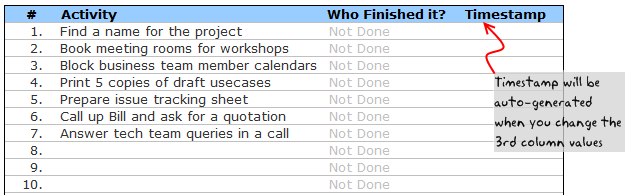
- First we will create a to-do list in excel in the following format:
Note, depending on the type of project and the kind of activities involved, your team to do list can look differently.
- In order to facilitate tracking, we have the following features:
- A column where the team member can specify his / her name. This should be done when the activity is done. A simple alternative could be to automatically load user’s name based on windows login ID. For more on this, see this article on DDoE.
- Another column where we generate a time stamp when the user enters the name. Please read this article to generate time stamps in excel
- The formula for time stamp is like this:
=IF(AND(D6<>"Not Done",D6<>""),IF(E6="",NOW(),E6),""). As you can guess, it is a circular formula. So we should enable iterative calculations from calculations options in Excel. Learn more about circular references here. - Using above 2 columns, we can track and measure how team members are working various activities and who has done what.
- When we are done, the todo list for project tracking looks like this:

- Once the list is created, first we should save it a network location where the list can be accessed by everyone.
- If your team is spread across the globe and cannot access one network, try the following options,
- Use Excel 365, it supports shared spreadsheets
- Sharepoint, If you have a sharepoint site that can be accessed by everyone, post the file there
- Use google docs spreadsheets. Google docs spreadsheets is a free alternative to MS Excel with several collaboration and team features. It is very intuitive and simple to use.
- You can create multiple copies of the to do list and share it with your team members and consolidate all the spreadsheets on frequent basis. This is a painful process as any format changes can create problems to your consolidation process.
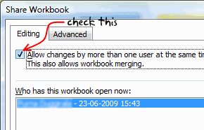
- Once you place the file on network, we should enable sharing of the workbook. See the below screenshots to understand how to share a workbook.

- Now go get some work done.
- When you finish the task, just open the shared workbook and mark the task as done by entering your name. Excel will automatically fill in the time stamp when you marked the activity as done.
Download the To Do List Template and Use it to track your projects
Go ahead and download the excel team to-do list template and use it as a project tracking tool.
Download 24 Project Management Templates for Excel
Next Steps
You can use VBA macros to automatically remove the finished to do items. I have written an article on simple to do list app using excel sometime back. Check it out to get some ideas.
In the next installment, learn how to prepare a project time line that can display various key project milestones. If you haven’t already, read the previous part of the project management using excel series – Project Planning using Gantt Charts.
Resources for Project Managers
Check out my Project Management using Excel page for more resources and helpful information on project management.
Your thoughts and suggestions?
I am not a project management expert. In fact, I know very little about project management, that is why I started this series, so that I can share the little I have picked up in the last few years and learn more from you. Please tell me your feed back using comments. I would love to hear from you.


5 Responses to “Preparing Profit / Loss Pivot Reports [Part 2 of 6]”
[...] Preparing Pivot Table P&L using Data sheet [...]
[...] Preparing Pivot Table P&L using Data sheet [...]
[...] Preparing Pivot Table P&L using Data sheet [...]
I am not getting sound from the videos. I have checked all the settings and spent several hours searching the Internet to no avail.
Has anyone else had this problem?
Is there anyway to get the Grand Total to be broken out in the same fashion as the items above it? For instance, if you have in column 1, widget a, widget b, and have their sales by month in column 2, I'd like to see the grand total also be by month, for widget a & b combined.
I can't get anything other than a single line for the grand total, rather than the same format as the data above.
Widget A Month Sales
Jan 100
Feb 200
Widget B
Jan 150
Feb 250
Grand total - here I would also like to have Jan, Feb.
Jan 250
Feb 450