Today we will learn Excel SUBTOTAL formula and 5 beautiful reasons why you should give it a try.
SUBTOTAL formula is used to find out subtotal of a given range of cells. You give SUBTOTAL two things – (1) a range of data (2) type of subtotal. In return, SUBTOTAL will give you the subtotal for that data.
Unlike SUM, AVERAGE, COUNT etc. which do one thing and only one thing, SUBTOTAL is versatile. You can use it to sum up, average, count a bunch of cells.
Here is the SUBTOTAL syntax:
=SUBTOTAL (TYPE OF TOTAL, RANGE OF CELLS)
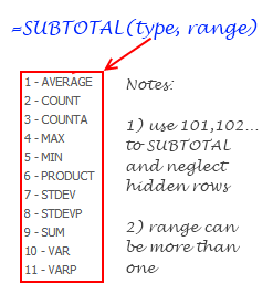
So, for example, =SUBTOTAL(9,A1:A10) will give us the sum of all values in A1:A10, provided none are filtered(more on this filtering thing below). That is because “9” stands for SUM in SUBTOTAL lingo. If you want a count of values, you can use “2”.
Hmm, that sounds like any other formula, what is so special about it?
Well, SUBTOTAL is not just any other formula, it is a special one. We don’t need to be Jedi masters to tell that force is with SUBTOTAL.
Here I have listed 5 reasons why this is such a special formula.
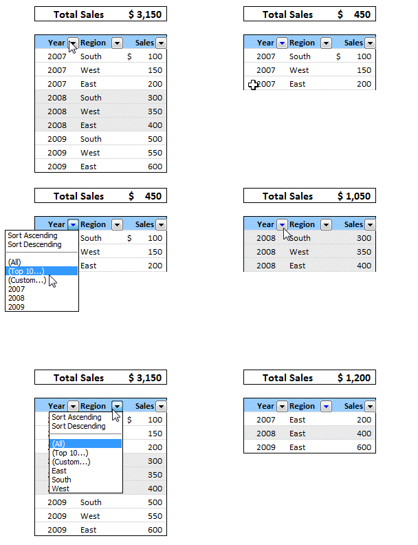
1) You can use SUBTOTAL to find sum of filtered values
I think the title says it all. See this example to know more.
2) You can use SUBTOTAL to ignore values in hidden rows
Often, we use hide rows feature in excel to remove irrelevant items from view. You can use SUBTOTAL with special type codes so that values in hidden rows are neglected.
For eg. SUBTOTAL(9,A1:A10) finds the sum of values in cells A1:A10 where as SUBTOTAL(109,A1:A10) will find sum of values in visible rows only.
3) You can use SUBTOTAL to dynamically summarize data
Since the “type of total” is a parameter to SUBTOTAL, we can use that to make a dynamic summary like this:
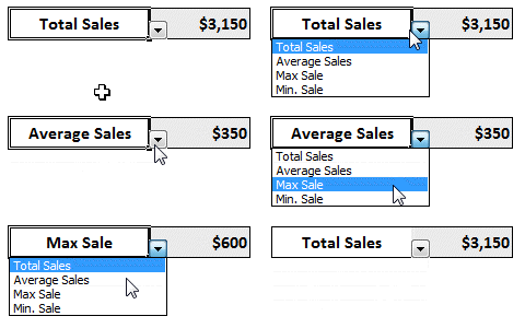
This is very handy in dashboards or when you don’t have space for everything.
4) If there are subtotals in SUBTOTAL range, they will be neglected
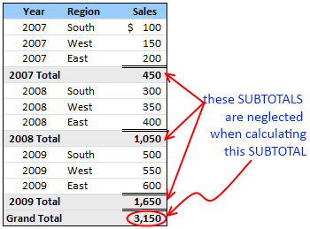
This is a killer feature of SUBTOTAL. If you have any SUBTOTAL formulas in the input range of another SUBTOTAL formula, these values are neglected so that double counting is avoided. Need I say more?
5) You can automatically create SUBTOTALs using Excel Data Tools
While SUBTOTAL formula looks kind of neat, writing them when you have tabular data can be a drag. But you don’t have to worry about that. In Excel’s Data menu / ribbon, there is an option on called “Subtotals” that automates the whole process for you.
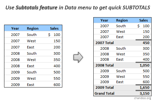
To generate automatic SUBTOTALS, just select your table of data, go to Data ribbon (or menu) and click on “Subtotals”. This will launch a Subtotal dialog where you can easily specify the type of total grouping you want.
That simple!
Related Excel Formulas:
SUMPRODUCT | VLOOKUP | SUMIF & COUNTIF
Have you used SUBTOTAL formula?
I have never really bothered to test SUBTOTAL formula until few days ago. Now that I found some really cool uses for it, I am itching to implement some of them in future. What about you? Have you used SUBTOTAL formula before? Do you got any tips to share? Please use comments to discuss.


32 Responses to “Extract Numbers from Text using Excel VBA [Video]”
Interesting that you are posting this at the same time as Doug http://yoursumbuddy.com/regex-function-sum-numbers-string/
Looks like two different articles about two different subjects, extracting numbers in text vs. summing all the numbers in text. Also, articles are published 20 days apart. Is the interesting part that there were two articles written about Visual Basic techniques within this month?
Sorry, that should have said 1 day, not 20. Was looking at the wrong thing. I still think it's just a nice coincidences to have multiple articles about VB written. Dick Kusleika also routinely writes about VB at dailydoseofexcel.com
What a lucky coincidence. I know about Doug's blog, but havent had a chance to read it in a while. Thanks for sharing the link.
I think that the best lesson that can come from the several salary survey solutions is that one should have anticipated the variety of monetary units. If the survey utilized drop down currency lists and limited the salary field to whole numbers only, etc. the resulting input would have been far cleaner. Sorry, Chandoo, but the messy input was, in my opinion, self-inflicted.
You are right. Since there are more than 200 different currencies, I thought a currency field would complicate the survey. The bigger problem was, Google Docs (which I used for survey) does not have an option to capture only numbers. Input fields were by text, so people entered in lots of different formats.
But I am happy how it turned out. It taught me several lessons on how to clean data.
Next time I will use a better tool to capture such responses.
Your post made me check how the "regular" and "irregular" decimal separators look like in different countries and it appears to be really interesting case. Take a look:
http://en.wikipedia.org/wiki/Decimal_mark
Cheers.
I am pretty sure you can replace this code block from your article...
If Text Like "*.*,*" Then
european = True
Else
european = False
End If
with this single line of code...
european = Format$(0, ".") = ","
Just to follow up on my previous post, I think I may have misunderstood the intent of your code. You were not looking to see if the computer system was using a dot for the decimal point, rather, you were looking to see if the Text was using a dot as the decimal point, weren't you? If so, then you could use this single line of code as to replace your If..Then..Else block...
european = Text Like "*.*,*"
But what if the number in Text was not large enough to display a thousands separator? Or what if it were a whole number? In either of those cases your original test, and my replacement for it, will fail. Maybe this would be a better test...
european = Right(Format$(Text, "."), 1) = ","
You are right. I am checking if the text has European format. And I loved your one line shortcut. I did not think of using LIKE in such context. Thanks for sharing that.
Again, you are right that this method would fail if the number is not big enough for a thousands separator. Since my data has annual salaries, all numbers are usually in thousands. So I did not think about it.
Hi ,
I have a question please. I'm working on a report that has alphanumeric on it and I only need to retrieve 7 integers that starts with 7 and 3 example SCM RIS PX RIS 02 - 7152349, ADSF\243434134, CM532345 and i need to get the 7152349. Can you please help me on this? I truly appreciate your help!
Thank you very much!
Hi-
The post was wonderful. Please take a look at this function also
Function ExtractNumber(InputString As String) As String
'Function evaluates an input string character by character
' and returns numeric only characters
'Declare counter variable
Dim i As Integer
'Reset input variable
ExtractNumber = ""
'Begin iteration; repeat for the length of the input string
For i = 1 To Len(InputString)
'Test current character for number
If IsNumeric(Mid(InputString, i, 1)) Then
'If number is found, add it to the output string
ExtractNumber = ExtractNumber & Mid(InputString, i, 1)
End If
Next i
End Function
Thank you so much. Your function code is amazing. It very useful for my lesson. Thank you so much.
To be more international.
At the beginning, for the rench format :
If fromThis.Value Like "*.*,*" Or fromThis.Value Like "* *,*" Then
european = True
End If
And at the end :
ElseIf ltr = "," And european And Len(retVal) > 0 Then
retVal = retVal & Application.DecimalSeparator
End If
Hi Chandoo,
Sorry, but your code does not work correctly with my Hungarian excel. My decimal separator is "," so
getNumber = CDbl(retVal)
will not convert the string to value, because you hard-coded "." as separator.
And, as you mentioned: "method would fail if the number is not big enough for a thousands separator" I would like to add: would fail if the user did not enter the thousand separator and also would fail if the thousand separator is not "," nor "." but " " (space chr) - as in Hungary.
This two functions could help to determine the system settings:
application.DecimalSeparator
application.ThousandsSeparator
Conclusion:
you say: "We do not need special treatment for regular format (61,000.30) as Excel & VBA are capable of dealing with these numbers by default." - it is true in case you system uses the regular format. 🙂
Cheers,
Kris
Awesome! It works !!
But how does one take into account negative numbers (say the list has negative numbers and I want to retain those negative numbers)
Thanks.
Hi. When I download this example, my excel is not showing formulas exactly. I wanted a ready version of this example, please. Thank you
Hi Chandoo,
Thanks for this brilliant article like many others that you have written for the benefit of many. Unfortunately, I am constantly having problems downloading your sample workbooks. I am currently using Excel 2007, and each time I try to download any of your sample workbooks, for e.g. the 'Extract Numbers Using VBA workbook', I get the following message 'This file is not in a recognizable format'.
I always get this message each time I try to download any of your sample workbooks. Please kindly advise me on how to resolve this.
Thank you.
Kenny
I have numbers like 12345-12-1 which I want to extract from text strings. 12345 might be variable there as 123, 1234, 12345, 123456,1234567 or so. When I get that in other cell (Column) I should see multiple entries of similar numbers with - (hyphen). How to do that?
@Madhav
Assuming your data is in cell A1
=LEFT(A1,FIND("-",A1)-1)
Thanks Hui for your response. Thank you for your time to find potential solution for my problem.
I tried your formula but was not successful in using the same.
here is more clarification so that you/others could help me.
Column A has following in Cells A1 to A4.. could be long..
ABCD 12345-12-1 XYZ 9878-02-9
LMNOPQ 12345-12-1 STQ 789748-98-5
NFHFKDJFKDS 123-23-1, NDKANSD
A FDSAFNDS 12345-12-1, ASNDSAND
from such data I need to extract the number with hyphens
remove , immediately after the numbers, separate the numbers with spaces
Column B shall look like:
12345-12-1 9878-02-9
12345-12-1 789748-98-5
123-23-1
2345-12-1
2 separate strings (numbers) having hyphen (-) therein should be separated with space.
@Madhev
Have a look at a solution using a simple UDF
https://www.dropbox.com/s/zexf4t9tmxmt3m9/Get_Numbers.xlsm?dl=1
Thanks Hui that worked well with the examples I provided.
I should have given following type of example:
2-ABCD 12345-12-1 X-2-YZ 9878-02-9
in the above case I do not want to extract a number and hyphen which is connected to or is part of text string..
Can you please help me modify the code to ignore numbers and - with text string.?
Thanks in advance.
@Madhav
So what is the answer expected from
2-ABCD 12345-12-1 X-2-YZ 9878-02-9
Thanks for your interest and time Hui.
so when I have text like
2-ABCD 12345-12-1 X-2-YZ 9878-02-9 3-abc-4-efg in Cell A2
in B2 the answer should be only numbers with hyphens and no text with numbers or hyphens
12345-12-1 9878-02-9 OR
12345-12-1 some delimiter (, or 😉 9878-02-9
The logic I thought was (but unable to do)
1. remove all strings containing text (and - and numbers) and then extract only numbers containing hyphens
2. Extract numbers in only following format ( # is a digit below) and ignore numbers and hyphens in any other format
#######-##-#
######-##-#
#####-##-#
####-##-#
###-##-#
##-##-#
Hope this helps.
Why not just use the function =getNumber ?
=getnumber doesn't extract numbers with hyphens..
also need to ignore numbers and hyphens associated with text string
When I use this code that code give me error
cdb1 is not highlight can u explain me
@Deepak
It runs fine for me
Select the first line and Press F9 to set a stop point
goto a cell and edit the function and press Enter
Then you can step through the code when it runs using F8
report back what happens
HI,
How can we add spaces between numbers and removing decimals.
how can we make spaces in the reesult e.g 25 655 2335
Dear Team,
I need to extract number (cheque number) from a cell (some numbers may repeat that to be ignored),
Text is - :-Inward Clg Cheque 00992924 00992924,BD
Result should be - 992924
Kindly help in getting formula for this (please email the code or VBA Code)