Dear Readers & Friends,
I am very happy to announce that Excel School online training program is now available for your consideration. Please read this short post to understand what you will get when you sign-up for this program and how you can join.
What will you get when you join?
- Access to Private Member-only Classroom: Where you can learn, ask questions, share ideas and discuss home work & class projects.
- Weekly Excel Lessons for 12 weeks: Includes Videos, Demos, Animations, Excel Workbooks
- Downloadable Lessons: You can download the lessons once every 4 weeks so that you can learn at leisure
- 2 Class Projects: Where you will build a Dynamic chart and a simple dashboard based on the techniques taught in the program
- 3 Bonus Weeks: Apart from the 12 weeks of regular training, I have 3 bonus weeks planned on (1) Excel Shortcuts and Productivity (2) Macros (3) Form Controls. This bonus content will be released in parallel with regular content so that the program duration is not changed.
- Excel Formula Cheat-sheet: This one page PDF file can act like a quick reference for Excel Formulas.
- Useful Excel Shortcuts – Cheat-sheet: Print this one pager and stick it near your desk. You will never have to search for most-common key board shortcuts.
- Complimentary Access to Member area even after the course ends. That is right. The entire course contents, neatly structured by week will be available for access, download and discussion even after 12 weeks are over. You can access all the content for 6 more weeks. Membership gives you access for 22 weeks. So even if you are busy and missed few weeks of the program, you can always comeback and learn at leisure.
Important things to keep in mind:
- I will close the Excel School registration and payments on 17th Feb, 2010. No new members will be added after that. So if you want in, you better hurry.
- Classes will begin on 22nd Feb, 2010 and go on until last week of May. You can watch all the lessons, continue discussions until 4th of July.
- This program is not for absolute newbies. The words ‘formula’, ‘reference’, ‘chart’ should ring a bell for you. If not, this program is not for you.
Pricing & Payment Options
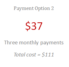
You have two payment options. You can either pay one time or pay three monthly payments.
(please visit this page if you cannot see the payment buttons in your e-mail or feed reader)
|
![]() |
|
![]() |
||
What happens after you “add to cart” ?

Note: If you are not redirected to “registration page” after payment, pls. don’t freak out. I will send you an email with your login details with in 24 hours
More Details:
For a more detailed copy, visit the Excel School Sales Page. You can also find a sample lesson, detailed contents and more info there.
If you have some questions about the program, please check out the Excel School FAQs. Also, try posting a comment here and I will get back to you.
I am very eager to see you in Excel School and help you become better in MS Excel.
PS: Expect some Excel School ads and mentions on the blog for next 10 days.
PPS: Regular broadcast of Excel tips and awesome stuff starts tomorrow.
PPPS: Go ahead and sign-up for Excel school already.


15 Responses to “Compare 2 Lists Visually and Highlight Matches”
Hi,
I solved this in a little different way.
We have 2 lists, one starts at A1 and other at B1, both are vertical arrays.
First thing is define 2 named ranges, list1 and list2:
list1 refers to "=OFFSET(Sheet1!$A$1;0;0;SUMPRODUCT(--(Sheet1!$A$1:$A$1000""));1)"
list2 refers to "=OFFSET(Sheet1!$A$1;0;0;SUMPRODUCT(--(Sheet1!$B$1:$B$1000""));1)"
this way lists will be dynamically sized when you had or remove elements (you can't have blanks and you can't have more than 1000 elements).
Then I use conditional formatting in column A when this formula is true:
"=NOT(ISERROR(MATCH(A1;list2;0)))"
and "=NOT(ISERROR(MATCH(B1;list1;0)))" to list2.
This way we eliminate the need for auxiliary columns or lists.
Hope you like my way! 😀
Nunes
Simple conditional formatting formula.
Assuming lists vertical lists starting in A1 & B1
To highlight just one column (assume B for example)
Conditional formatting>New Rule>by formula
=MATCH(B1,$A$1:$A$99,0)
Set the cell fill to what ever color you prefer & press OK
To highlight both columns repeat with this formula for cell in column A
=MATCH(A1,$B$1:$B$99,0)
This approach doesn't require named fields or addtl columns
glw
Say I had 1 list in A2:A20 and another in B2:B20.
To format all the items in column A that are repeated in column B I would use the following Conditional Formatting rule.
=IF(ISNA(VLOOKUP(A2,$B$2:$B$20,1,false)),true,false)
All the duplicates are highlighted. It us a very simple example of comparison.
I may be missing something here, but I usually highlight both my lists by holding ctrl eg A1:A20 E10:E40 then choose conditional formatting from the ribbon and then highlight duplicates, and this does it?
Lee, I was perplexed as well. I do the same thing you do with the conditional formating. A drag and click to highlight range and choose highlight duplicates does the trick for me.
I believe these methods are to check if an item from one list also appears in the other list. So if an item mentioned many times in one list if also mentioned in the other list or not.
The Conditional Formatting highlight duplicates feature will do this, but it will also highlight an item if it appears multiple times in the one column or list.
Hi, I would just like to know (if you are willing to share) which image editing program you use to make your image like above, like they are torn apart from bottom? I've been looking for long.
@i48998
Chandoo is on Holidays, but Chandoo uses Paint.Net
Paint.net is a free download available at http://www.paint.net/
.
I use CorelDraw/PhotoPaint
.
We both use the Snipping Tool (a freebe with Win Vista/10)
.
We both use Camtasia for doing screen captures to make animated GIFs where you see animation.
Here is how I would accomplish
(1) Define Names: List_1, List_2
(2) =ISNA(MATCH(D4,List_2,0))-1 (Conditional Format formula List_1)
(3) =ISNA(MATCH(D4,List_1,0))-1 (Conditional Format formula List_2)
ISNA will return 1 if NO Match and O if Match by adding a -1 will make: NO Match 0 and Match a -1 which is True
Hi all
this my first Post here
i think we can take Unique List for tow list to know what is not Duplicate By this Array formula
=IFERROR(INDEX($D$6:$D$33,SMALL(IF(ISERROR(MATCH($D$6:$D$33,$B$6:$B$33,0)),ROW($D$6:$D$33)-ROW($D$6)+1),ROWS($J$5:J5))),"")
and this one for Duplicate Value
=IFERROR(INDEX($D$6:$D$33,SMALL(IF(ISNUMBER(MATCH($D$6:$D$33,$B$6:$B$33,0)),ROW($D$6:$D$33)-ROW($D$6)+1),ROWS($J$5:J5))),"")
Don't forget to Enter This Formula by Pressing Ctrl+Shift+Enter
without wanting to ruthlessly self promote here, I do have an addin that does neatly compare two ranges, not just in columns, so you might want to check that out.
Having said that this is a pretty neat solution if you dont want to be going down the VBA or purchase route. I like it
however, could you not do something with the remove duplicates feature in Excel 2010 and then compare the resulting data set?
Hi, Chandoo! I've found yesterday your Excel website... What can I say? It's just awesome, Excellent. Being a developer for 30 years, more than 15 with Office products, and wow!, how many things I discovered in a couple of hours, and what pretty resolved.
I decided to take the long path of the newbies and read all your examples and write down by myself all of them, and when I arrived to this (the comparison of two lists) I think I've found a problem:
a) in "Step 4: Apply conditional formatting to Second List - Use the same logic, but this time the rule becomes =COUNTIF(count1s,$H6)" it should say "Step 4: Apply conditional formatting to Second List - Use the same logic, but this time the rule becomes =COUNTIF(count1s,$H6)>0", but this is a typing error that I believe all of us here might have discovered and corrected
b) the very problem: I wrote down two different lists, in different ranges, and with different number of elements, I specified the equivalent conditional formats, et non voilá!, I didn't get what expected. So I downloaded your example book, I checked range names, formulaes, conditional formats and all OK. So I copied -just values- from my book to yours, and I still couldn't achieve the goal.
I'm using Excel 2010 in spanish, I'm from Buenos Aires (Argentina), and my book is at your disposition whenever you considerate it appropiate.
Thanks in advance for your time, and again my congratulations for your work here.
Best regards.
SirJB7
Comparison of 2 lists visually with highlights
Author: SirJB7 / Date: 11-Dic-2011
Pros: no duplicated tables, no matrix formulaes, no named ranges, no VBA code, just conditional formatting
Cons: not found yet, comments and observations welcome
Features:
a) standard problem: highlights in orange/yellow elements existing in the other list
b) optimized problem: idem a) plus highlights in red/violet first occurrence of elements existing in the other list
Sheet contents:
a) conditional format, 1 rule per list (2 methods used)
A1:A20, first list
B1:B20, second list
a1) range A1:A20, condition =NO(ESERROR(BUSCARV(A1;B$1:B$20;1;FALSO))), format Orange ---> in english: =NOT(ISERROR(VLOOKUP(A1,B$1:B$20,1,FALSE)))
a2) range B1:B20, condition =CONTAR.SI(A$1:A$20;B1)>0, format Yellow ---> in english: =COUNTIF(A$1:A$20,B1)>0
b) conditional format, 2 rules per list (2 methods used)
D1:D20, first list
E1:E20, second list
b1) range E1:E20, condition 1 =Y(NO(ESERROR(BUSCARV(D1;E$1:E$20;1;FALSO)));COINCIDIR(D1;D$1:D$20;0)=FILA(D1)), format Red ---> in english: =AND(NOT(ISERROR(VLOOKUP(D1,E$1:E$20,1,FALSE))),MATCH(D1,D$1:D$20,0)=ROW(D1))
same range, condition 2 and format 2, same as a1)
b2) range E1:E20, condition =Y(CONTAR.SI(D$1:D$20;E1)>0;COINCIDIR(E1;E$1:E$20;0)=FILA(E1)), format Violet ---> in english: =AND(COUNTIF(D$1:D$20,E1)>0,MATCH(E1,E$1:E$20,0)=ROW(E1))
same range, condition 2 and format 2, same as a2)
Personally I like the a2) and b2) solutions, I think the formulaes are prettier.
I still don't know the rules of this website and forum, but it any precept is infringed I'm willing to share the workbook with the solution. If it breaks a rule, I apologize and promise that won't happen again.
Best regards for all!
Dear All i have a complicated situation...
1. I have two sheets of data Sheet1 and Sheet2 (from various sources) - Both of these contain data matching and Not matching as well..
2. Now for me i need to build an excel where in i need to get sheet 3 with values that are present in a column of Sheet 1.
What ever Sheet 1 doesn't have i dont want those rows from sheet 2 to be populated into Sheet3.
Can any one help me out.
Hi Team
The above example is to compare partial name from 2 different columns.
If I want to cross check it in a single column. I have both correct and partial correct/match entries in a column. Is there any way I can find both the entries in the column.
Regards