


Conditional formatting is one of favorite features in Excel. CF has helped me save the day at work more than a dozen occasions. I almost became project manager just because I knew how to make a gantt chart in excel using conditional formatting. I have written extensively about it.
So, I was naturally curious to explore what is new in Excel 2010’s Conditional Formatting. In this post, I will share some of the coolest improvements in CF.
1. You can refer to data in other worksheets now

This is the best new addition to CF capabilities in Excel 2010. Now we can refer to data in other worksheets without using any named ranges or copying the data over to primary sheet.
2. Solid Data Bars, Finally!
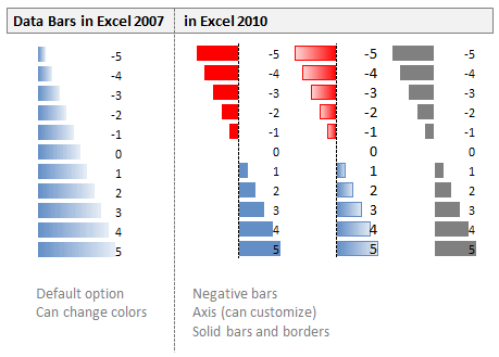
In Excel 2007, MS introduced a new feature called “data bars”. It felt like an exciting thing, except for one gnawing problem. The bars have gradients. So, not only they looked ugly, but they were also difficult to read (also, they were inaccurate at default settings).
Thankfully MS rectified these problems and significantly improved data bars in Excel 2010.
Now, you can,
- Create data bars with solid fill
- Apply borders to data bars (so that even gradient fills look elegant)
- Have negative data bars
- Have an axis so that comparison is easy
Here is a small comparison between Excel 2007 & Excel 2010 Data Bars:
Using data bars to create in-cell progress charts:
You can use data bars to create in-cell progress charts (or thermo-meter charts) like this:
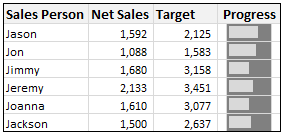
* Hint: The trick is to use cell background color along with data bar.
[Related: Jon Peltier has written a beautiful article reviewing data bars in Excel 2010.]
3. More Icon Sets in Conditional Formatting
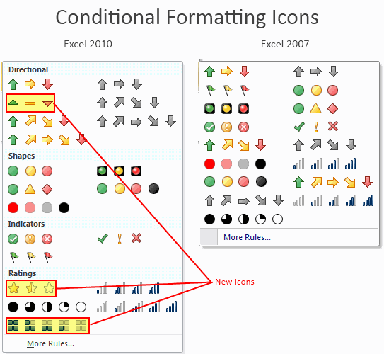
Although I rarely use icons in conditional formatting, I am happy to report that MS has added 3 new sets of Icons to the conditional formatting library.
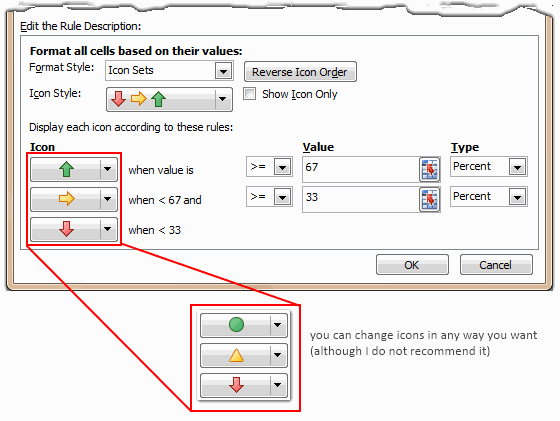
Also, you can mix and match icons depending on the rules (how I wish they didnt allow this. Mix and match can produce more evil combinations than good ones.)
What do you think about new CF Features in Excel 2010?
I am excited to try the data bars in real-world project. I find the possibility of referring to other sheets very good. Also, I am not sure if its just me, but Excel 2010 conditional formatting feels fast. In fact, not just CF, almost everything in Excel 2010 feels fast and responsive.
What about you? How are you planning to use Excel 2010 CF features in your work? Please tell us using comments.
PS: By leaving a comment, you can win a copy of Office 2010 – Home & Student Edition. Contest sponsored by Microsoft India.
References: Excel Conditional Formatting Improvements [MSDN blog]
Related: Excel 2010 – What is new? | Overview of Excel 2010 Sparklines


49 Responses
The Good, the No Longer Bad, and the Ugly.
1. Allowing references to another sheet is always nice. Of course, you could always use the same trick that enabled data validation between sheets, that is, name the cell whose value you wanted to use in a condition. So this is a small advance.
2. Nice, they got it right this time.
3. Just what we needed, more bling. It wasn’t bad enough with all the new gradients, fills, shadows, glows, and the small number of icon sets that 2007’s cat dragged in.
I ended up here by googling “Excel 2010 weird”, getting what I expected, lots of frantic people. It has taken a simple concept – the spreadsheet – and turned it into a Cretan labyrinth. And I have no idea why it takes hourglasses of time to open an empty spreadsheet. Do they just want you to look at the logo, like advertising?
Perhaps Microsoft gets its input from upper-level management, which, looking for ways to pass the time, has fun deriving new appearances for everything – rather than from actual office workers, who are trying to enter data meaningfully.
@Greg
Excel is setting up lots of things in the background when the Logo is being displayed
Better to have you look at that than start to try to do something when it isn’t ready and then you will be frustrated at the slow response
If you really want to speed up loading I’d suggest installing excel on a SSD drive on your PC as they allow applications to load super fast
ps: Office Vista was terribly slow loading, so upgrading may also be an option. My Office 2010 loads in about 1.25 seconds, Excel 2013 in about 2.5 seconds.
Intruiging! I will look into this SSD Drive.
If I use this correctly, look nice and be informative. Good improvement.
Great article as always. I really like #2 : solid bars, negative data bars, axis for comparison, etc… They finally got it right compared to 2007! I will definitely use this feature once I get Excel 2010.
I wonder if the solid bars could be turned into bullet charts with any ease.
And come on Jon, a _little_ bling never killed anyone:)
I quite liked the data bars in 2007, but I only used a few times. They work well if your data is all positive, but now that I see the 2010 version, I’m looking forward to it.
Rob
I can’t wait to try these built-in additional functionnalities and stress them in rea
I can’t wait to try these built-in additional functionnalities and stress them in real life. By the way, Fabrice Rimlinger, author if SFE (Sparklines for Excel) did a review comparison you can access it here : http://sparklines-excel.blogspot.com/2010/02/sparklines-for-excel-vs-excel-2010.html
(damn IE cut short myfirst reply).
There is so much value to conditional formatting. I love the fact that you can now reverse the icon sets to match your liking. When working on KIP’s, an up arrow could be green for one thing and red for another….. etc. Another positive change to the ’07 version.
Good improvement on Solid Data Bars. However, still looks bad the axis values overlaped by the bars. Should be more flexible….
Nice Icon Sets. All the improvements in the CF are more than welcome!! Very used feature by all…
Reference to data in other worksheets is nice to have but I still think that named range is more professional and I do recommend it as a best practice.
Improvemnts and advancements always welcomed by me. I cant wait to have Excel 2010.
Reference of other sheet in Conditional formating seems good. Change in Icon set as you like is also good.
@Jon Peltier,
Thanks for the tip about 2007. I didn’t realize that we can name a cell in a different sheet and use it in Conditional Formatting.
Will definitely try that.
Subhash
Speed / responsiveness improvement is always good ! In some cases 2007 was really slow.
@Jon peltier
indeed thanks for the hint to use a reference to a different sheet in the conditional formatting, I will try this it helps !
This article really whets my appetite…
The big question for me is how backwards-compatible are the 2010 conditional formatting options. Half of the people I work with are still using Excel 2003!!!
Mark –
Conditional Formatting is not at all backwards compatible with 2003 and earlier versions. When you open a fancy new workbook in 2003, you get a message that tells you that certain options are not available.
Because of these incompatibilities and the fact that many customers and clients are still only up to 2003, I have yet to make use of conditional formatting or such things as the new functions in 2007 (sumifs, etc.).
These comments are based on Excel 2003…. I have a love/hate relationship with conditional formatting. I love it because, applied sparingly, it is very useful in highlighting important drivers of the information within context of the analysis environment. However, from a practical point of view, sharing a conditionally formatted table is difficult. You have to make sure to include external indexing references (if any) on the same sheet you wish to share with other people; Printing to black and white printers of conditionally highlighted information usually results in visual chaos;
Also, I have noticed that these conditional formats spread like viruses (the unintended consequences of copy and paste actions) to other cells in the spreadsheet; And the management of conditional formatting is problematic with big conditionally formatted blocks of cells breaking down (sometimes) to individually listed lines in the conditional format manager (at least the remove all menu items solves for this issue).
bill
Couldn’t agree more with Bill. “CFs spread like viruses” is an apt phrase. It is not straight forward and not worth the effort yet to justify the new features, most of which I will never ever use. Does anyone have any useful tips for setting CF on pivot tables and for a grid of approx 150 rows by 50 columns which will not cause the package to lock up and lose your work as you attempt to paste the format in? Is it to do with setting a range? If so how do you stop the viral aspect from changing other cells when the condition is not applicable to them?
Hi Chandoo, I like your review.
Regarding Mark comment, I would like to stress the point that a lot of people is still using Excel 2003.
Moreover, the enhancements 2007 to 2010 are not so significant as those 2003 to 2007
For them, I would like to celebrate the new functionality…
One of the features I love the most of the new Excel Conditional formatting is the ability to apply formatting relative to a group of cells; this way you can find/show relationships between them (data bars, icons, color scale). We have the option “Format all cells based on their values” in addition to “Format only cells that contain” of 2003 version.
Additionally, the Conditional Formatting Rules Manager is worth mention too. Not new in Excel 2010 but many 2003 users maybe don’t know the benefits:
* Now you can see/edit the range that the rules apply to
* Now you can move up/down each rule so you change the order in which the rules apply (so simple now but a not so straightforward process in Excel 2003)
* That’s not all, you can choose which workbook rules to show: selection, sheet, etc
I wrote an article that covers the enhancements since 2003, it complements the article of Chandoo here.
These are my reasons to use Excel 2010 CF (from a 2003 user point of view)…
1) I love Excel 2010 Conditional Formatting because it has a new friendly user interface
2) I love Excel 2010 Conditional Formatting because it has pre-built formatting options
3) I love Excel 2010 Conditional Formatting because it has more rules and you can now move them up and down and more…
4) I love Excel 2010 Conditional Formatting because it has 4 new rule types (conditions)
http://www.excel-spreadsheet-authors.com/excel-2007-conditional-formatting.html/
1. I don’t know how many times I have wanted to reference cells in other sheets. This will save me a lot of setup time since now I will not have to put the formula in each CF.
I wish I had 2010 to play with so I could check out all this stuff. 🙁
Solid Data Bars are much appreciated in conditional formatting.
I like conditional formatting and I use it quite often, but I don’t use all the bells and whistles in my work. Many times in 2007 I want to use C.F. on adjacent cells with different criteria, but because they’re adjacent, somehow they get “connected”. argh! Hopefully this is corrected in 2010
A great future, AND either MS missed something or I’m missing something…
Let’s say I make A1’s formatting dependant on the value of B1. As I change the value of B1 Excel does not automatically update the formatting of A1 – the only way I can get Excel to update the formatting of A1 is to ‘F2’ or edit A1 … any thoughts, suggestions, ideas?
@Bennie.. Thanks for the comments and welcome to Chandoo.org.
Did you have manual calculation mode on? That could result in such peculiarity.
@Bennie
If Chandoo’s idea doesn’t help, is your Spreadsheet telling you that it has a Circular Reference error at the lower left corner of the screen
One of the more frustrating things about conditional formatting was that a user could not manually change formatting that was already Conditionally formatted. For example, say I prepared a conditional format to make cells with values higher than 3 turn green background. If i tried to manually change one of the green backgrounds to red (perhaps to temporarily indicate an error), it will not work; the cell will remain green. The cell will remain green until the CF is removed from that cell. Does Office 2010 address this problem?
does anyone how to use conditional formatting with icons for both positive and negative values. i.e. I want the green light icon to be present when a value exceeds 10%(positive) or drops below 10% (negative). right now, I can only figure out how to use it if above 10% (positive)
@Renee
Add another series which will have =NA() when not applicable and hence be hidden
and have the appropriate value/symbol when required.
Have a read of: http://chandoo.org/wp/2010/11/11/highlight-data-points-scatter-line-charts/
This is good, but…do you know how to conditionally format a bullet within an XY scatter chart?
@Greg
You can’t Condiftionally Format a data point without using the technique above point #26 or vba
Is there a way to get the colors reversed? I’ve got data (moving average) for which I want to add the context of the average the same period before the moving average. In this case higher means not good, so I would want to have an up arrow signalling the greater average, but in a red color since its a bad thing.
Any ideas?
when I apply conditional formatting for icon sets, I lose all text ib the 2nd of 3 pages! I remove conditional formatting and I have all three pages back. Frustrating to not have use of such an otherwise great tool…
in the previous post, ib = on
This might be a really dumb question but … how does Excel calculate the percents for the distribution for the icon sets? What total is used? I would like to use the icon sets in a table but I cannot understand how the distribution has been calculated and the colours/icons on the default % distribution are not what I calculated using the total. I would appreciate some help with this. Thanks very much for your time.
@Kim
Thats a very good question, which I can’t answer.
Firstly, I rarely use icons, but investigated them for this question
I setup 4 cells which added to 100
the first cell adjusted its value so I could change the others but the total; remained 100
I had CF Icon Rules >=67% and >=33%
the Orange Flat icon didn’t change to a Green Up Icon until the cells value was >75% of the Highest value, this was about 22% of the total
So I can only assume that internally MS has used some sort of distribution, rather than a straight 67% of the total or highest value
Thanks very much Hui – thats what I did when I failed to figure it out (and I ran alot of other descriptive statistics tests as well). I was trying to visualise school enrolment ratios and the stakeholders love the icons which like you I never use. Must be something in that natural aversion …
I was looking for information on Excel2010 and conditional formatting improvements when I came upon this page. It is a good overview. I wish to be able to change the CF of a cell to another color but the value in the cell never changes. I use this for a visual form of progress and evolution of a chart that each cell represents a pixel and a fixed value. It is a spatial tool. Presently, I have to manually change the cell’s color and five colors takes a bit of time to update in a 7 x 10 cell grid. The grid begins with no colors and each CF represents an event in time. Older events get changed to a different color as they are updated. Kind of like a Petri Dish from day to day.
Maybe there is a way to do this now, I am still looking.
How about a format rule based on color?
“Conditional formatting is one of favorite features in Excel. CF has helped me save the day at work more than a dozen occasions. I almost became project manager just because I knew how to make a gantt chart in excel using conditional formatting. I have written extensively about it.” Really???????? You “almost” became a PM? LOL!
Jeff York, PMP
Does anyone know if I can add my own icon sets for conditional formatting?
@Fredrik
Bad news buddy, You can’t
It is a glaring deficiency in Excel amongst several others
Since switching from 2007 to 2010, any table previously created in 2007 loses its conditional formatting for “if this cell is greater than this cell, format with bold and shading”. All my shading for cells greater than the first cell has disappeared and even if you completely remove the formatting in the entire table and start again it no longer works. Very frustrating. Any suggestions?
Hi
I need to know how to do the following for a test and cannot work out how. Could someone please help and write down the steps to do the following “Specify cell values in the bottom 33% will not display an icon”
Many thanks
Fleur
Hi
Use Conditional Formatting under the Home tab menu. By default, you have orange, green and red color Icons. For the values < 33%, click the arrow bottom to select No Icon option.
Hope it helps
Vafa