
Occasionally we deal with data that is so uncooperative that we might as well give up and go back to calculators & ledger books.
Recently I found myself in such a situation and learned something new.
Introducing … data that won’t play nice
Drum roll please. Here is a data-set that I got from somewhere.
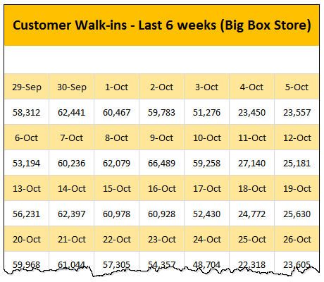
The problem – build a lookup formula
And the problem. Oh, simple. Write a lookup formula to find how many customer walk-ins we have on any given day.
But how?
After wrestling with a few variations of VLOOKUP, INDEX, MATCH, OFFSET… I found the right formula for this occasion.
SUMIFS Formula
That’s right, the good old (well, its just 7 years old, born in 2007 Excel) is the one that works in this situation.
Assuming our data is in the range:
- B4:H15
- Even rows (4,6,8…14) containing date
- Odd rows (5,7,9…) containing customer walk-ins
- And lookup date is in L5
We can use this SUMIFS formula:
=SUMIFS(B5:H15,B4:H14,L5)
to find out how many customers walked in to the store on the lookup date.
How does this formula work?
See this illustration.
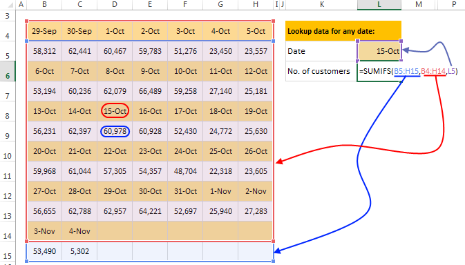
Since SUMIFS (and SUMIF too) formula works in 2D, our formula works elegantly.
Any caveats?
There are a couple of problems with this formula.
- It works for looking up numbers only
- It doesn’t work if any of the numbers are same as dates we are looking up. For example 15th October 2014 is 41927, so we have a data point that is also 41927, then our SUMIFS result would be wrong.
A better formula?
If you want a formula that works with any type of data, then of course we can come up with one.
That is your home work.
Go ahead and figure it out and share your magic potions in the comments.
Here is a clue: If we cant go somewhere directly, we can go indirectly, if we know the address.
Download Example Workbook
Click here to download the example workbook. Examine the formula in cell L6 to understand how this works.
How do you deal with such data?
Badly shaped data is everywhere. Not a week goes by when I don’t come across poorly structured data. Thanks to Excel, I can alter the shape of almost any data. My favorite techniques are – text import, power query, formulas, pivot tables, remove duplicates & go to special.
What about you? How do you deal with poorly structured data? What tools do you deploy to alter the fitness levels of your data? Please share your thoughts and tips in comments.
Don’t forget about the formula challenge.
Excel not co-operating? Its time you tamed it
Data that is messy, bosses with high expectations, coffee machines that don’t work are everywhere. Fortunately Excel can fix 2 of those 3 problems. (Sorry folks, there is no fixCoffeeMachine() macro, yet.)
Learn a few Excel tricks & concepts and you could be on your way to taming messy data & demanding bosses. Start with these:


7 Responses to “Build models & dashboards faster with Watch Window”
yes, I use watches in excel vb
Dear Chandoo,
This is a quite useful for myself. I highly appreciate your efforts for acquainting us with this value adding and time saving tip.
I'll admit it, I never saw this feature before. I was familiar with using Watch Window in VB, but not in workbook. I'll definitely use this in future when building dashboards!
it was always great reading your blog, one thing that i want to know, which tool you are using to create such gif image?
it was also a nice post,,,,,, sir
Hello Sir,
Really very nice post. I didn't use this features in past. But now going to use it..
Thanks a lot for every time come up with something new..
Thanks
Very Nice post sir.
Every Time posting something new.. Thanks a lot