How to present changes in Market Share using Charts?

Share

Facebook
Twitter
LinkedIn

Most of us are comfortable with numbers, but we are confused when it comes to convert the numbers to charts. We struggle finding the right size, color and type of charts for our numbers. The challenge is two fold, we want to make the charts look good (we mean, really… really good) but at the same time we want our audience to focus on the message and not on the bells and whistles. This is where it gets tricky.

Almost 2 months ago our reader Jennifer sent me an email asking if there is an effective way to present market share changes between two periods for 2 products among five competitors.  I have replied her promptly with whatever I could think of as better ways to present the data. But I also posted a visualization challenge: How to show market share changes?

We have got quite a few comments and recently Jon Peltier himself wrote on this here: Show Market Share Changes – Few Alternatives

I thought it would be great to summarize various approaches we discussed as a case-study in how you can take same data and present it in different ways.

This is the data Jennifer had:

Market Share Data - Excel Charting Problem

  1. Here is how she presented it initially:
    market-share-product-2
  2. After seeing user discussions she remade the charts like this.
    Stacked Bar chart and lines showing market share
  3. Derek from Information Ocean responded to the challenge with this step graph (which he admits is not so effective). Nevertheless, they are another fun alternativeStep chart - market share
  4. Derek also proposed this “who is responsible for that?” chart. Despite looking little cluttered I liked this one.
    Line chart - Who is responsible for that?
  5. Dave from Favillae responds with this aligned bar chart alternative to present the same data. Another innovative way, he used blank series to adjust the gaps
    Aligned Bar Charts
  6. Nixnut, a commenter, tried bar charts to come up this variation. These are pretty good and provide both absolute and changes in market share values. He used overlapped chart technique to achieve this.
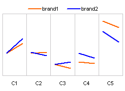
    Bar Charts
    (image url)
  7. Finally the alternatives presented by Peltier.
    This one is a panel chart
    (here is an excel tutorial for panel charts)
    Panel Chart
  8. A stacked bar chart
    Stacked Bar Chart
  9. A line chart
    Another Line chart
  10. A simpler, neater bar chart
    Simple Bar Chart
  11. A panel chart, but this time two products are separated
    Panel Chart with 2 Panels
  12. Last but not least, these are the alternatives I could think of. First one is a Line chart.
    Another Line chart
  13. This is a tag cloud (excel tag cloud tutorial & templates). The fonts are sized based on their relative market share percentages.
    Tag Cloud
  14. And in-cell chart variation.In-cell Chart

Conclusions – Which chart is better?

Well, there were quite a few very good charts. Personally I liked the panel chart version (#7) and bar chart variation by NixNut (#6).

Which one did you like?

Knowing that there are various ways to present the same data and using the version most suitable for your needs and situation is very important. If you want to raise alarm about market share loss, use a chart that alarms people. If you want to downplay the marketshare loss, use a chart that barely shows the information.

Facebook
Twitter
LinkedIn

Share this tip with your colleagues

Excel and Power BI tips - Chandoo.org Newsletter

Get FREE Excel + Power BI Tips

Simple, fun and useful emails, once per week.

Learn & be awesome.

Welcome to Chandoo.org

Thank you so much for visiting. My aim is to make you awesome in Excel & Power BI. I do this by sharing videos, tips, examples and downloads on this website. There are more than 1,000 pages with all things Excel, Power BI, Dashboards & VBA here. Go ahead and spend few minutes to be AWESOME.

Read my storyFREE Excel tips book

Overall I learned a lot and I thought you did a great job of explaining how to do things. This will definitely elevate my reporting in the future.
Rebekah S
Reporting Analyst
Excel formula list - 100+ examples and howto guide for you

From simple to complex, there is a formula for every occasion. Check out the list now.

Calendars, invoices, trackers and much more. All free, fun and fantastic.

Advanced Pivot Table tricks

Power Query, Data model, DAX, Filters, Slicers, Conditional formats and beautiful charts. It's all here.

Still on fence about Power BI? In this getting started guide, learn what is Power BI, how to get it and how to create your first report from scratch.

15 Responses to “Compare 2 Lists Visually and Highlight Matches”

  1. Nunes says:

    Hi,
    I solved this in a little different way.

    We have 2 lists, one starts at A1 and other at B1, both are vertical arrays.

    First thing is define 2 named ranges, list1 and list2:
    list1 refers to "=OFFSET(Sheet1!$A$1;0;0;SUMPRODUCT(--(Sheet1!$A$1:$A$1000""));1)"
    list2 refers to "=OFFSET(Sheet1!$A$1;0;0;SUMPRODUCT(--(Sheet1!$B$1:$B$1000""));1)"

    this way lists will be dynamically sized when you had or remove elements (you can't have blanks and you can't have more than 1000 elements).

    Then I use conditional formatting in column A when this formula is true:
    "=NOT(ISERROR(MATCH(A1;list2;0)))"
    and "=NOT(ISERROR(MATCH(B1;list1;0)))" to list2.

    This way we eliminate the need for auxiliary columns or lists.

    Hope you like my way! 😀

    Nunes

  2. glw says:

    Simple conditional formatting formula.
    Assuming lists vertical lists starting in A1 & B1
    To highlight just one column (assume B for example)
    Conditional formatting>New Rule>by formula
    =MATCH(B1,$A$1:$A$99,0)
    Set the cell fill to what ever color you prefer & press OK

    To highlight both columns repeat with this formula for cell in column A
    =MATCH(A1,$B$1:$B$99,0)

    This approach doesn't require named fields or addtl columns
    glw

  3. Alan says:

    Say I had 1 list in A2:A20 and another in B2:B20.

    To format all the items in column A that are repeated in column B I would use the following Conditional Formatting rule.

    =IF(ISNA(VLOOKUP(A2,$B$2:$B$20,1,false)),true,false)

    All the duplicates are highlighted. It us a very simple example of comparison.

  4. Lee says:

    I may be missing something here, but I usually highlight both my lists by holding ctrl eg A1:A20 E10:E40 then choose conditional formatting from the ribbon and then highlight duplicates, and this does it?

  5. Greg says:

    Lee, I was perplexed as well. I do the same thing you do with the conditional formating. A drag and click to highlight range and choose highlight duplicates does the trick for me.

  6. Alan says:

    I believe these methods are to check if an item from one list also appears in the other list. So if an item mentioned many times in one list if also mentioned in the other list or not.

    The Conditional Formatting highlight duplicates feature will do this, but it will also highlight an item if it appears multiple times in the one column or list.

  7. i48998 says:

    Hi, I would just like to know (if you are willing to share) which image editing program you use to make your image like above, like they are torn apart from bottom? I've been looking for long.

  8. Hui... says:

    @i48998
    Chandoo is on Holidays, but Chandoo uses Paint.Net
    Paint.net is a free download available at http://www.paint.net/
    .
    I use CorelDraw/PhotoPaint
    .
    We both use the Snipping Tool (a freebe with Win Vista/10)
    .
    We both use Camtasia for doing screen captures to make animated GIFs where you see animation.

  9. Rick says:

    Here is how I would accomplish
    (1) Define Names: List_1, List_2
    (2) =ISNA(MATCH(D4,List_2,0))-1 (Conditional Format formula List_1)
    (3) =ISNA(MATCH(D4,List_1,0))-1 (Conditional Format formula List_2)

    ISNA will return 1 if NO Match and O if Match by adding a -1 will make: NO Match 0 and Match a -1 which is True

  10. Hi all
    this my first Post here
    i think we can take Unique List for tow list to know what is not Duplicate By this Array formula
    =IFERROR(INDEX($D$6:$D$33,SMALL(IF(ISERROR(MATCH($D$6:$D$33,$B$6:$B$33,0)),ROW($D$6:$D$33)-ROW($D$6)+1),ROWS($J$5:J5))),"")
    and this one for Duplicate Value
    =IFERROR(INDEX($D$6:$D$33,SMALL(IF(ISNUMBER(MATCH($D$6:$D$33,$B$6:$B$33,0)),ROW($D$6:$D$33)-ROW($D$6)+1),ROWS($J$5:J5))),"")

    Don't forget to Enter This Formula by Pressing Ctrl+Shift+Enter

  11. Excel Addin says:

    without wanting to ruthlessly self promote here, I do have an addin that does neatly compare two ranges, not just in columns, so you might want to check that out.

    Having said that this is a pretty neat solution if you dont want to be going down the VBA or purchase route. I like it

    however, could you not do something with the remove duplicates feature in Excel 2010 and then compare the resulting data set?

  12. SirJB7 says:

    Hi, Chandoo! I've found yesterday your Excel website... What can I say? It's just awesome, Excellent. Being a developer for 30 years, more than 15 with Office products, and wow!, how many things I discovered in a couple of hours, and what pretty resolved.
    I decided to take the long path of the newbies and read all your examples and write down by myself all of them, and when I arrived to this (the comparison of two lists) I think I've found a problem:
    a) in "Step 4: Apply conditional formatting to Second List - Use the same logic, but this time the rule becomes =COUNTIF(count1s,$H6)" it should say "Step 4: Apply conditional formatting to Second List - Use the same logic, but this time the rule becomes =COUNTIF(count1s,$H6)>0", but this is a typing error that I believe all of us here might have discovered and corrected
    b) the very problem: I wrote down two different lists, in different ranges, and with different number of elements, I specified the equivalent conditional formats, et non voilá!, I didn't get what expected. So I downloaded your example book, I checked range names, formulaes, conditional formats and all OK. So I copied -just values- from my book to yours, and I still couldn't achieve the goal.
    I'm using Excel 2010 in spanish, I'm from Buenos Aires (Argentina), and my book is at your disposition whenever you considerate it appropiate.
    Thanks in advance for your time, and again my congratulations for your work here.
    Best regards.
    SirJB7

  13. SirJB7 says:

    Comparison of 2 lists visually with highlights
    Author: SirJB7 / Date: 11-Dic-2011
    Pros: no duplicated tables, no matrix formulaes, no named ranges, no VBA code, just conditional formatting
    Cons: not found yet, comments and observations welcome
    Features:
    a) standard problem: highlights in orange/yellow elements existing in the other list
    b) optimized problem: idem a) plus highlights in red/violet first occurrence of elements existing in the other list
    Sheet contents:
    a) conditional format, 1 rule per list (2 methods used)
    A1:A20, first list
    B1:B20, second list
    a1) range A1:A20, condition =NO(ESERROR(BUSCARV(A1;B$1:B$20;1;FALSO))), format Orange ---> in english: =NOT(ISERROR(VLOOKUP(A1,B$1:B$20,1,FALSE)))
    a2) range B1:B20, condition =CONTAR.SI(A$1:A$20;B1)>0, format Yellow ---> in english: =COUNTIF(A$1:A$20,B1)>0
    b) conditional format, 2 rules per list (2 methods used)
    D1:D20, first list
    E1:E20, second list
    b1) range E1:E20, condition 1 =Y(NO(ESERROR(BUSCARV(D1;E$1:E$20;1;FALSO)));COINCIDIR(D1;D$1:D$20;0)=FILA(D1)), format Red ---> in english: =AND(NOT(ISERROR(VLOOKUP(D1,E$1:E$20,1,FALSE))),MATCH(D1,D$1:D$20,0)=ROW(D1))
    same range, condition 2 and format 2, same as a1)
    b2) range E1:E20, condition =Y(CONTAR.SI(D$1:D$20;E1)>0;COINCIDIR(E1;E$1:E$20;0)=FILA(E1)), format Violet ---> in english: =AND(COUNTIF(D$1:D$20,E1)>0,MATCH(E1,E$1:E$20,0)=ROW(E1))
    same range, condition 2 and format 2, same as a2)
    Personally I like the a2) and b2) solutions, I think the formulaes are prettier.
    I still don't know the rules of this website and forum, but it any precept is infringed I'm willing to share the workbook with the solution. If it breaks a rule, I apologize and promise that won't happen again.
    Best regards for all!

  14. sunil says:

    Dear All i have a complicated situation...

    1. I have two sheets of data Sheet1 and Sheet2 (from various sources) - Both of these contain data matching and Not matching as well..

    2. Now for me i need to build an excel where in i need to get sheet 3 with values that are present in a column of Sheet 1.

    What ever Sheet 1 doesn't have i dont want those rows from sheet 2 to be populated into Sheet3.

    Can any one help me out.

  15. Jagdev says:

    Hi Team

    The above example is to compare partial name from 2 different columns.

    If I want to cross check it in a single column. I have both correct and partial correct/match entries in a column. Is there any way I can find both the entries in the column.

    Regards

Leave a Reply