
Here is a quick tip to start the week.
Often, we end up with a situation where a bunch of numbers are stored as text.
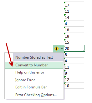
In such cases, Excel displays a warning indicator at the top-left corner of the cell. If you click on warning symbol next to the cell, Excel shows a menu offering choices to treat the error.
Converting numbers stored as text back to numbers
Tip #1: Error correction
One easy and quick way to convert all the text-numbers to numbers is,
- Select all the cells
- Click on warning indicator next to top-most cell
- Choose Convert to number option
- Done
Tip#2: Paste Special Convert
Sometimes such text-numbers may be scattered across the worksheet, thus making selection of cells a pain.
In such cases, follow this process (see demo below)
- In a blank cell, just type 1
- Copy this blank cell.
- Select all the cells that have text-numbers.
- Press CTRL+ALT+V to launch Paste Special box.
- Choose Multiply from operation area.
- Click ok & Done!
Enjoy your numbers.
Bonus tip: If you think the error indicators are annoying, you can turn them off. Just go to File > Options > Formulas and turn off all the error checking rules you don’t need.
PS: Thanks to Justin for emailing me the Paste Special Multiply with 1 trick.


43 Responses
Additional tip,
Select column which contains text -> Data -> Data tools -> Text to columns -> Finish
Chandu
This one is particularly awesome if you have tens of thousands of data to convert to number. Otherwise it can take excel forever (minutes to half hour or longer) to process an error correction.
This is definitely the best option, and has the added benefit that you can use it to convert text to numbers, and numbers to text, depending on whether you choose General or Text before clicking Finish!
when you use this method it’s worth making sure that there are no delimiters selected (just in case)
another method is to do a find & replace (I routinely use zero with zero, or . with .)
ALT+A+E>>enter>>enter will do it 🙂
OMG Thank you Chandu! I was struggling with this so much with my big datasheets and now I am so happy! so funny.
In my excel though, it is the same pattern but it is:
1) Choose the data tab
2) highight the column you want to change
3) choose “text to columns” in the ribbon
4) select fixed width
5) enter
6) no crashes!!
Often the text which you want as a number will have a decimal point, so Select column which contains text -> Data -> Data tools -> Text to columns ->Select apostrophe to add also as the delimiter -> Goto Advanced and add the decimal point. -> Finish, Voila. It works. You can then format as currency etc. Worked in Ver 2013. Seems that MS is degrading some important functions so as to get users to upgrade to 365.
Sir, how convert text to number in Power Query.
I had never thought about multiplying the numbers by 1 before. Great tip. For those who love macros, I found a very well written VBA macro by Ejaz Ahmed (StrugglingToExcel.com). This macro not only converts the numerical text to numbers but also formats dates and trims the values (getting rid of those nasty leading/trailing spaces). Plus you can apply this to multiple columns at the same time! I immediately added it to my QAT bar and use it almost daily with my data extracts. Check it out!
http://www.thespreadsheetguru.com/the-code-vault/2014/8/21/convert-numbers-stored-as-text
This tip is awesome! But one thing I run into constantly is the need to convert text to number and keep the leading zero, if there is one. I work a lot with SSNs and zip codes, etc. Any help, much appreciated!!
Hi Sue,
let ur zip code (length 5) in Column B, then select Column B and go to ‘Format Cell’ (CTRL + !) – Number – Custom – enter 00000 in Type field.
Now put, 15 in cell B1 and it will show 00015.
Hope this will solve ur query.
1) SSNs and ZIP codes are not numeric. They are meant to be character based identifiers. With numbers, leading zeros to the left of the decimal are not significant and are truncated. It may sound terribly picky of me to bring up the distinction, but I’ve learned that it does make a difference in some cases. (Especially when delivering to a client who is attempting to extract and then load your data into a different DBMS.)
2) The option described by SAURABH below (custom format, 00000) will work in Excel but it’s only displaying the number as ‘00015’ while the actual value of the cell will still be 15 because you have converted it to a number and excel will pay attention to significant digits (see above.) Meaning, if you “Paste special” with values only into a new cell, it will paste ’15’ into the cell rather than ‘00015’, which could lead to problems depending upon how you need to carry them into new work. Your client’s ETL process may bring in ’15’ rather than what you intend ‘00015.’ I usually leave SSNs and ZIP as text, that way leading zeros (and dashes in the case of SSNs) are preserved.
Better than #2 (don’t waste time dirtying and clearing a cell)… Copy a blank cell (really blank, not containing anything), select cells to change, Paste Special Values, Operation Add.
+1. Excellent tip.
An alternative to multiplying the numbers by 1 is to add 0 instead by using the same process as the multiplication method. At least you can save a step. You don’t have to enter a 1 to multiply. The blank cell is 0 and can be added to change text to a number.
One thing I find very handy when doing this, as I often have intermittent numbers as text:
Select the first cell that has the warning flag, then ctrl-down arrow to the last one. Once you have it all, especially if it’s thousands of cells, it’s annoying to scroll back up to get to the flag. If you apply formatting, such as setting the cell fill color to none, it automatically takes you back up to the top without losing your selection.
Good Tips !
I knew both the tips before. I like the tip mentioned by “Jon Peltier”. Amazing + Awesome 🙂 He steals the Show .. I mean this Post 🙂 😉
Thanks for contribution to all !
Regards,
Rahim Zulfiqar Ali
Love this post. I often have to export SAP Reports to excel and then do various sorts and lookups. This text issue has been driving me crazy. I especially like Jon Peltiers method where we can add a blank cell via paste special. Will be forwarding this tip to my friend Michael Martin.
yes, Michael Martin was impressed!
I also benefitted from Ctrl Alt V to paste special. I don’t know how I have missed this one all these years. This is something we do a lot around here.
Hi again! One reason I asked about the leading zero is not so much for display purposes. I realize that ’15’ formatted to ‘00015’ still has a value of ’15’. That is one of my issues!! I receive data from multiple sources and need to constantly do look-ups and queries, and I drive myself crazy trying to format the different spreadsheets so they can ‘talk’ to each other. Does anyone have a tried and true process for syncing up columns where numbers are stored as text? For me, it’s SSN, personel number, and zip. And, I think some of the sources they ARE number and some (like our DB queries) come in as text. aaargh. And, thank you in advance.
Ah, I see. I’d format anything ZIP or SSN related to text, and then clean up my lookup tables to be in that format as well. To convert those ’15’s back to ‘00015’s there are two ways that I use.
1) If I’m reformatting an entire workbook, I actually DO use the custom format to adjust some columns, like zip codes or dates in an unusual format (like ’21 Aug 14′, etc.) when I have everything like it needs to be, I save the result as a .CSV file. When excel saves a custom format as .CSV, it defaults to value (the display option) and discards value2 (the underlying actual value.) Text files have no record of formats, they are lean by their nature, so when you open it, Excel will attempt to interpret each column. Because of this, I close the CSV, and I use the text import wizard, (Data Tab > “From Text”) to bring in the CSV. The import wizard lets me specify which columns I want to be Characters and which I want to be numbers, (and it does dates as well for good measure.)
2) If I’m only able to reformat a single column, I’ll usually do that via a Macro, for example, if the zip codes have had their zeros truncated by excel, I format that column as text, and run this “padding” macro that I wrote for that purpose:
Sub Pad_to_X()
On Error Resume Next
‘This will insert zeros in front of a number.
‘X is the length of the entire number plus zeros
‘so if you have 1 and want 001, X would be 3
With Application
.DisplayAlerts = False
End With
x = InputBox(“Enter X, and the selection will be padded with leading zeros to X characters”)
For Each cell In Selection
lenc = Len(cell)
diff = x – lenc
If diff > 0 Then
padme = Empty
For nn = 1 To diff
padme = padme & “0”
Next nn
cell.Value = padme & cell.Value
End If
Next cell
With Application
.DisplayAlerts = True
End With
End Sub
Cleaning data from multiple sources is fun. Often a lookup will bomb because the table or the dataset has characters that mean something to the client’s software (or webpage,) but are “invisible” when you look at them in excel. In those cases, I recommend trimming leading and trailing whitespace, and looking for and removing chr(160) (HTML Non-Breaking whitespace.) Those are the most common.
Sometimes the character in a cell is something you’ve never considered, and in the cases where a value isn’t found in a lookup table, I’ll run this “decode string” macro to split out the cell value and display it by its ASCII equivalent. It’ll identify any weird relics, which you can then sweep for with a cleaning macro:
Sub Decode_String()
Dim sttrarray(1 To 5000) As Variant
Dim sttrarray2(1 To 5000) As Variant
‘instring = InputBox(“String to Decode?”)
instring = Selection.Value
lenstring = Len(instring)
count = 0
For x = 1 To lenstring
sttrarray(x) = Asc(Mid(instring, x, 1))
sttrarray2(x) = Mid(instring, x, 1)
count = count + 1
Next x
Workbooks.Add
targ = ActiveWorkbook.Name
sht = ActiveSheet.Name
Workbooks(targ).Sheets(sht).Range(“A1”).Value = “Position”
Workbooks(targ).Sheets(sht).Range(“B1”).Value = “Character”
Workbooks(targ).Sheets(sht).Range(“C1”).Value = “ASCII decode”
For n = 1 To count ‘
Outp = Outp & “Position ” & n & ” is ” & sttrarray2(n) & ” or chr ” & sttrarray(n) & Chr(13)
Workbooks(targ).Sheets(sht).Range(“A” & n + 1).Value = n
Workbooks(targ).Sheets(sht).Range(“B” & n + 1).Value = sttrarray2(n)
Workbooks(targ).Sheets(sht).Range(“C” & n + 1).Value = sttrarray(n)
Next n
End Sub
Multiply 1, divided by 1, add or subtract 0 all do the trcik… ;p
Select the column and hit ALT+D+E and Finish till dialogue box disappears. We are good to go
Instead of typing 1 and copying it, just copy any blank cell and go to paste special and add.
It happens that I need to attach some data from external source over and over again and the data comes in text format. If these procedures are too difficult, I use extra column to have values in numbers. The formula is very simple: =value()
You go from “sometimes text-numbers may be scattered across the worksheet, making selection of cells a pain.” to “3. Select all the cells that have text-numbers.”
You just said it’s a pain to select the cells… so you instruct us to do it anyway? Am I the only one who fails to see logic here?
@Belgianbrain:
You dont have to individually select such cells. you can select entire range that contains such data and do it. That is what I mean by “Select all the cells”
Good Tips! Thanks for sharing, very useful when SAP reports must be exported
Put zero in a cell >> Copy >> Paste Special >> Add
…will also do that.
Awasome… Chandooo..
But if data is too large u can use the Function =Value( & Then Use Paste Special.
Else this trick is superb.
Love this website!!!!
The “enter 0”, copy – paste special – add method puts a zero in blank cells.
Similarly, for the enter 1- copy paste special multiply.
The copy blank – copy – paste special – add method does not seem to have this drawback.
Thank you.
If you do use the first option (click on ‘Convert to number’) and you’re working in a large model, make sure you turn on the Manual calculation mode. Otherwise Excel will recalculate after each converted number. This can be really annoying if a model takes 0.1 seconds to recalculate and you just told Excel to convert a couple of thousand numbers!
The Value() formula works fine as well, which is good for external data, or to be used in LOOKUP functions. The other way around, by the way, if you must LOOKUP a value and you’re looking it up in an array of text values, I use =TEXT(A1,”0″) to convert a value to its string equivalent.
I also love the Add 0 tip, I hadn’t thought of that!
Really a useful tip,for me my users use SAP as input where often tedious to select all the cells and again go to the top row to convert numbsers.
Really a very useful tip.
To those keyboard people:
To access this “error handling menu”, press the Alt + Right Click Button, then press the “C” to convert to number… this last “C” is in portuguese, I dunno what the equivalent in english is.
Also another thing I learned together with this trick. If you are using one of these new keyboard, that doesn’t have a Right Click button, the equivalent to it is Shift + F10… so it would be Alt + Shift + F10 then “C”
This tip (Tip#2: Paste Special Convert) saved my life! I’ve always done all my conversions the 1st way. Working across multiple sheets exported from my Accounting program, all the zeros are always listed as text. It was so frustrating – and then this tip came along! Thank you thank you thank you! I now just select all sheets, do the ctr+alt+v thing and voila! all text is now zeros!
Very very useful tip 🙂
Chandoo Tu Bhai hai
Thanks a lot
Hi All,
I have few data with month as column name and Planned hours, forecast for months,actuals hours , ETC as Row data. What I want is whenever the user enter values in forecast month(Current month) , it shld color the cells.and when the user enter the values in Actuals hours(it will be of prevous month) it shld fill the color.The cycle will continue . Also As the month will pass on the previous valued cells shld be in no format.
https://www.youtube.com/watch?v=IbVwhrfegcI
My excel crashes to the point it is unusable. The only method I have found that wont crash my machine is find & replace (replace 1 with 1, and so on.) I am not sure what causes this in my sheets, and it can even cause another machine to start having this issue. I assume it is settings or the data itself. I created a dump file off the process before crashing, which ended up being huge. Looking in the file with notepad, some data I can’t see. But towards the bottom of the file there is a ton of words – waiting on word wrap to finish in it to see what it says.
@aly
a few things
What type of PC is it?
How much RAM?
What version of Windows/Excel are you using ?
Do you know how many lines of data you have ?
Can you ask the question in the Chandoo.org Forums?
https://chandoo.org/forum/
Please attach the data file so we can give you more specific help