Christmas Gift Shopping List Template – Set budget, track your gifts using Excel

Share

Facebook
Twitter
LinkedIn

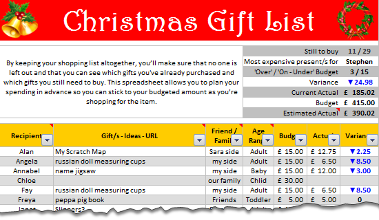
Last year, Steven shared a beautiful Christmas Gift List template with all of us. It is packed with lots of Excel goodness. Just a few days ago, he emailed me another copy of his file with some improvements. So if you are planning for Christmas shopping and want a handy tracker, you don’t want to miss this.

Christmas Shopping List Template using Excel

How does this template work?

This template feels magical. To begin with,

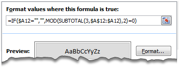
Zebra lines thru Conditional Formatting

Alternative rows of the template are shaded in dull gray color so that the template is easy to use. And this is achieved by Conditional Formatting & SUBTOTAL formula. A very ingenious use of SUBTOTAL formula so that the zebra lines preserve even after filtering data.

Zebra Lines using Conditional Formatting

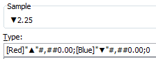
Custom Cell Formatting to Show Budget vs. Actual Variance

Another simple yet elegant solution. To highlight the variance between budgeted & actual gift value, Steven used Custom Cell Formatting.

Custom Cell Formatting rules to highlight budget variance

Awesome Formulas to Summarize the Gift List

The top right area of Steven’s shopping list shows a clear summary of your Christmas shopping list. Each of the values in the summary are calculated by a clever formula. For example, the formula to show how many gifts are over the budget vs. how many are on or under the budget is an intricately woven SUMPRODUCT formula with SUBTOTAL, OFFSET & ROW components. Go ahead and examine these formulas to learn more.

You can filter the list and analyze by segment

The beauty of this template is that you can filter the list and analyze by segment. For example, you can filter all the gifts you are giving to friends and see whether you are with-in budget in that segment, the progress of gift selection & purchase etc. Very useful.

Download Christmas Gift Shopping List Template

Click here to download the template and use it.

Go ahead and Enjoy your Christmas shopping.

Thanks to Steven

for sharing a beautiful & awesome template with all of us.

How do you like this template?

I really loved the simplicity and elegance of this template. It is easy to use, packed with lots of details and fun to poke around.

What about you? Do you like this template? How do you organize your Christmas spending? Do you use Excel, some other tools or rely on your gut feel? Please share using comments.

More Templates on Christmas & Thanksgiving

We, at chandoo.org celebrate holiday season by sharing useful templates, tips & ideas with you all. Here is a collection of holiday stuff for you:

Facebook
Twitter
LinkedIn

Share this tip with your colleagues

Excel and Power BI tips - Chandoo.org Newsletter

Get FREE Excel + Power BI Tips

Simple, fun and useful emails, once per week.

Learn & be awesome.

Welcome to Chandoo.org

Thank you so much for visiting. My aim is to make you awesome in Excel & Power BI. I do this by sharing videos, tips, examples and downloads on this website. There are more than 1,000 pages with all things Excel, Power BI, Dashboards & VBA here. Go ahead and spend few minutes to be AWESOME.

Read my storyFREE Excel tips book

Overall I learned a lot and I thought you did a great job of explaining how to do things. This will definitely elevate my reporting in the future.
Rebekah S
Reporting Analyst
Excel formula list - 100+ examples and howto guide for you

From simple to complex, there is a formula for every occasion. Check out the list now.

Calendars, invoices, trackers and much more. All free, fun and fantastic.

Advanced Pivot Table tricks

Power Query, Data model, DAX, Filters, Slicers, Conditional formats and beautiful charts. It's all here.

Still on fence about Power BI? In this getting started guide, learn what is Power BI, how to get it and how to create your first report from scratch.

21 Responses to “How to Filter Odd or Even Rows only? [Quick Tips]”

  1. Vijay says:

    Infact, instead of using =ISEVEN(B3), how about to use =ISEVEN(ROW())

    So it takes away any chance of wrong referencing.

  2. Hui... says:

    I like Daily Dose of Excel

  3. vimal says:

    I like it.

  4. Luke M says:

    Just a heads up, you do need to have the Analysis ToolPak add-in activated to use the ISEVEN / ISODD functions. An alternative to ISEVEN would be:
    =MOD(ROW(),2)=0

  5. Debbi says:

    rather than use a formula, couldn't you enter "true" in first cell and "false" in the second and drag it down and than filter on true or false.

  6. Paul S says:

    Just for clarification, is Ashish looking to filter by even or odd Characters or rows?

  7. Fred says:

    so many functions to learn!

  8. Istiyak says:

    Nice support by chandoo and team as a helpdesk. Give us more to learn and make us awesome. Always be helpful.......

  9. Arps says:

    In case you want to delete instead of filter,

    IF your data is in Sheet1 column A
    Put this in Sheet2 column A and drag down
    =OFFSET(Sheet1!A$1,(ROWS($1:1)-1)*2,,)
    (This is to delete even rows)

    To delete odd rows :
    =OFFSET(Sheet1!A$2,(ROWS($1:1)-1)*2,,)

  10. Pippa says:

    If your numbered cells did not correspond to rows, the answer would be even simpler:
    =MOD([cell address],2), then filter by 0 to see evens or 1 to see odds.

  11. Matthew D. Healy says:

    I sometimes do this using an even simpler method. I add a new column called "Sign" and put the value of 1 in the first row, say cell C2 if C1 contains the header. Then in C3 I put the formula =-1 * C2, which I copy and paste into the rest of the rows (so C4 has =-1 * C3 and so forth). Now I can just apply a filter and pick either +1 or -1 to see half the rows.

    Another way, which works if I want three possibilities: in C2 I put the value 1, in C3 I put the value 2, in C4 I put the value 3, then in C5 I put the formula =C2 then I copy C5 and paste into all the remaining rows (so C6 gets =C3, C7 gets =C4, etc.). Now I can apply a filter and pick the value 1, 2, or 3 to see a third of the rows.

    Extending this approach to more than 3 cases is left as an exercise for the reader.

  12. Paulo says:

    Another way =MOD(ROW();2). In this case, must to choose betwen 1 and 0.

  13. Makhan Butt says:

    very different style Odd or Even Rows very easy way to visit this site

    http://www.handycss.com/tips/odd-or-even-rows/

  14. Terhile says:

    Thanks for the tip, it worked like magic, saved having to delete row by row in my database.

  15. majid says:

    Thankssssssssssssssss

  16. Bhanu says:

    Hi Chandoo- First of all thanks for the trick. It helped me a lot. Here I have one more challenge. Having filtered the data based on odd. I want to paste data in another sheet adjacent to it. How can I do that?
    For Example-
    A 1 odd
    B 3 odd
    C 4 even
    D 6 even
    I have fileted the above data for odd and want to copy the "This is odd number" text in adjacent/next sheet here. How can I do that. After doing this my data should look like this
    A 1 odd This is odd number
    B 3 odd This is odd number
    C 4 even
    D 6 even

  17. Adriana says:

    Hi! Could you please help me find a formula to filter by language?
    Thank you!

  18. avinash says:

    Chandoo SIR,

    I HAVE A DATA IN EXCEL ROWS LIKE BELOW IS THERE ANY FORMULA OR A WAY WHERE I CAN INSTRUCT I CAN MAKE CHANGES , MEANS I WANT TO WRITE ONLY , THE FIG IS FRESH, BUT IN BELOW ROW IT WILL AUTOMATICALLY TAKE THE SOME WORDS FROM FIGS AND MAKE IN PLURAL FORM , WHILE USING '' ARE'' LIKE BELOW

    The fig is fresh - row 1
    Figs are fresh - row 2
    The Pomegranate is red - row 3
    Pomegranates are red - row 4

  19. Arshad Hussain Shah says:

    =IF(EVEN(A1)=A1,"EVEN - do something","ODD - do something else") with iferron (for blank Cell)

Leave a Reply