This is a guest post by Hui, our in-house excel ninja.
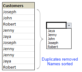
Here is a typical scenario: We want to allow only one of the pre-defined customer names in our spreadsheet. We have listed down all the customers in column B and want excel to check against this list and validate the data. But there are 3 problems. (1) Our list is not sorted alphabetically (2) It contains duplicates and (3) The list comes from external source, so we can not remove duplicates and sort the list every time.
Now how can we set up a simple data validation list that would not repeat customer names and shows them in sorted order like this:
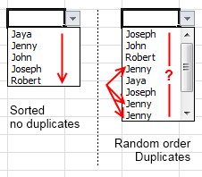
Here is the solution:
We need to remove duplicate entries and sort our data before it is fed to data validation list source. For this, there is a perfect tool right inside excel.
The rapid sorting cat.
Well, I am kidding. We use pivot tables. Pivot tables can sort the data as well as remove any duplicates. We can construct list of unique and sorted customers as column headers.
Just follow these simple steps:
- Select the source customer list and make a new pivot table. Insert the pivot table in the same sheet for convenience.
- Now, just add customer name to the column header area as well as “values” area.
- At this point, the column header in pivot contain all the customers (without duplicates) in sorted order.
- Now, make a dynamic named range that would refer to column headers in the pivot table. I am leaving this to your imagination, but here is a clue.
- Finally, use this dynamic range as input data source for data validation.
- That is all. Now, as and when your source data changes, just refresh the pivot and your validation will be updated too.
Note: You can make a dynamic range out of your input data as well. Or use excel tables if you have 2007 and above.
Download this example and learn by playing:
Here is an example sheet with a different data set (I use animals instead of customers).
Added by PHD:
Hui is an active member on PHD forums and helps people in solving excel problems. He likes to work on excel and has been kind enough to write this post in his free time to share such good idea with us.
Please say thanks to him if you enjoyed this post.
Learn more about data validations & duplicates:


15 Responses to “Christmas Gift List – Set your budget and track gifts using Excel”
[...] Christmas Gift List – Set your budget and track gifts using Excel … [...]
I'm confused: if you spend $10, and your budget is $40, shouldn't the amount in the "Within Budget?" column stay black, since you didn't go over budget?
In other words, since we overspent on the electronic photo frame, shouldn't the $8 cell turn red?
@JP.. maybe Steven is encouraging consumerism... ?
I havent realized it earlier, but now I see it. If you unprotect the sheet, you can change the formula in Column I to =IF(G13=0;" ";F13-G13) from =IF(G13=0;" ";G13-F13), that should correct the behavior.
Thanks Chandoo. I thought of making a shopping list spreadsheet for Christmas, but this is neat so I think I'll use this instead.
Chandoo & Steven thanks for this spreadsheet. But for the sake of a person who has been staring at this megaformula in vain for the last 40 mins and not afraid to ask, would it be possible for you to walk us through the logic used here?
=SUM(SUMPRODUCT(SUBTOTAL(3,OFFSET($K$13:$K$62,ROW($K$13:$K$62)-MIN(ROW($K$13:$K$62)),0,1)),--($K$13:$K$62="-"))+SUMPRODUCT(SUBTOTAL(3,OFFSET($K$13:$K$62,ROW($K$13:$K$62)-MIN(ROW($K$13:$K$62)),0,1)),--($K$13:$K$62="0")))&" / "&SUBTOTAL(2,$G$13:$G$62)
Thanks Chandoo.. This is one of the best budget spreadsheets I've ever seen.. The Arrays are out of this world!! And it's FREE!!
Chandoo, can you tell us more about Steven? Does he have his own site?
JP, I think Chandoo changed it when he changed the currency formatting from £ to $, a negative figure is a good thing in this case. But don't change the formulas, the overbudget and under budget won't work properly if you do. Also Chandoo I think you've accidentally broke the conditional formatting for the alternating row colouring the formula is different to the version I sent you. As for the megaformula chrisham, it gave me a headache trying to get it all working, so I will let Chandoo talk you through it.
Hi,
In cells I6 and I7, I understand that subtotal together with offset function returns an array of ones after which, the sumproduct function gives the desired result.
But I’m not able to figure out the reason for using an array in I8 to return the most expensive gift.
Can’t the formula be just
“=VLOOKUP(SUBTOTAL(4,$G$13:$G$62),$G$13:$J$62,4,0)”
Savithri, Cell I8 needs the array, if the formula was “=VLOOKUP(SUBTOTAL(4,$G$13:$G$62),$G$13:$J$62,4,0)” it would find the highest price from the filtered range (i.e. highest actual in filtered range is $50) BUT then return the first person with that actual, not looking in just the filtered range (so first person on the list with a $50 actual.)
To see what I mean, change the formula, then change all the actuals to $50 then filter for baby, it lists the first name on the list.
But a good question 🙂
Thank you. I now realise that the array is used to get the ‘filtered range’ instead of the entire range, as table array for look up value.
[...] Download This Template [...]
this looks like an awesome excel sheet!! is there anyway i can get it emailed to me unprotected? for some reason, i am unable to download it 🙁 help!!
Hi I also can not download to a mac as the sheet is protected any help would be great
[...] to send her a pricey present. Rather, send a card with a picture of your child. Here’s a cool Excel sheet that will help you estimate your budget per person and let you track [...]
[...] husband and I pour/poor over the Christmas spreadsheet (yes, I do know how dorky that sounds, but we’re not the only ones!), figuring out who should give what to whom. We live at a distance from most of our family, so it [...]