Thank you, Houston meetup & Bonus tip

Share

Facebook
Twitter
LinkedIn

My mom will be very unhappy with this post. She always told me to focus on one thing at a time. But in this post we are talking about 3 things, not one. Sorry mom.

1. Thank you

I want to thank you for visiting chandoo.org & supporting us.

As I am about to leave to USA for attending Excelapalooza conference, I couldn’t help but be amazed at how much you have given me & my family. Almost 4.5 years ago, when I left my plush corporate job to work full time on Chandoo.org, I had no clue how the future will unfold. Today my heart is full of happiness, my family is secure, my site has grown by heaps and our community (especially you) is awesome.

Without your enthusiasm to learn and keen desire to become awesome, I would not have a job (of running this website). You inspire me to learn new things everyday so that I can share them with you.

Thank you for all the visits, clicks, comments, emails, tweets, likes, signups, purchases & love.

Thank you.

2. Houston Meetup

I am in Houston between 15 – 19 September. If you live in or near Houston area, I would love to meet you, say thanks to you personally. So I have organized a meetup.

Venue: Arthur Storey Park (on Sam Houston Pkwy, Houston, 77072)

Time: Between 5 & 6:30 PM on Friday, 19th September

I will bring some snacks (don’t worry, healthy options only) and we can chat about all things Chandoo.org


Please click here to RSVP.


Special bonus for bicycle riders: If you ride your bike to the event, I will give you a free copy (ebook) of my VLOOKUP Book.

So go ahead and sign up.

3. Bonus tip

Here is a bonus Excel tip for you. Why? Because we are awesome like that.

Lets say you have a list of transactions in a table like this:

Sum values between 2 dates in Excel - howto?

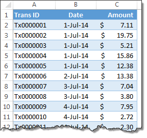
And you want to find out how much we made in month of July 2014?

You can use SUMPRODUCT to find the answer

Assuming the table is named trans

=SUMPRODUCT((trans[Amount])*(TEXT(trans[Date],"YYMM")="1407"))

Alternative formulas:

=SUMPRODUCT((trans[Amount])*(YEAR(trans[Date])=2014)*(MONTH(trans[Date])=7))

=SUMIFS(trans[Amount],trans[Date],">="&DATE(2014,7,1),trans[Date],"<"&DATE(2014,8,1))

For more on this technique, read Sum values between 2 dates.

So thats all for now. Enjoy your weekend.

And remember to signup for the Houston meetup if you are nearby.

Facebook
Twitter
LinkedIn

Share this tip with your colleagues

Excel and Power BI tips - Chandoo.org Newsletter

Get FREE Excel + Power BI Tips

Simple, fun and useful emails, once per week.

Learn & be awesome.

Welcome to Chandoo.org

Thank you so much for visiting. My aim is to make you awesome in Excel & Power BI. I do this by sharing videos, tips, examples and downloads on this website. There are more than 1,000 pages with all things Excel, Power BI, Dashboards & VBA here. Go ahead and spend few minutes to be AWESOME.

Read my storyFREE Excel tips book

Overall I learned a lot and I thought you did a great job of explaining how to do things. This will definitely elevate my reporting in the future.
Rebekah S
Reporting Analyst
Excel formula list - 100+ examples and howto guide for you

From simple to complex, there is a formula for every occasion. Check out the list now.

Calendars, invoices, trackers and much more. All free, fun and fantastic.

Advanced Pivot Table tricks

Power Query, Data model, DAX, Filters, Slicers, Conditional formats and beautiful charts. It's all here.

Still on fence about Power BI? In this getting started guide, learn what is Power BI, how to get it and how to create your first report from scratch.

21 Responses to “How to Filter Odd or Even Rows only? [Quick Tips]”

  1. Vijay says:

    Infact, instead of using =ISEVEN(B3), how about to use =ISEVEN(ROW())

    So it takes away any chance of wrong referencing.

  2. Hui... says:

    I like Daily Dose of Excel

  3. vimal says:

    I like it.

  4. Luke M says:

    Just a heads up, you do need to have the Analysis ToolPak add-in activated to use the ISEVEN / ISODD functions. An alternative to ISEVEN would be:
    =MOD(ROW(),2)=0

  5. Debbi says:

    rather than use a formula, couldn't you enter "true" in first cell and "false" in the second and drag it down and than filter on true or false.

  6. Paul S says:

    Just for clarification, is Ashish looking to filter by even or odd Characters or rows?

  7. Fred says:

    so many functions to learn!

  8. Istiyak says:

    Nice support by chandoo and team as a helpdesk. Give us more to learn and make us awesome. Always be helpful.......

  9. Arps says:

    In case you want to delete instead of filter,

    IF your data is in Sheet1 column A
    Put this in Sheet2 column A and drag down
    =OFFSET(Sheet1!A$1,(ROWS($1:1)-1)*2,,)
    (This is to delete even rows)

    To delete odd rows :
    =OFFSET(Sheet1!A$2,(ROWS($1:1)-1)*2,,)

  10. Pippa says:

    If your numbered cells did not correspond to rows, the answer would be even simpler:
    =MOD([cell address],2), then filter by 0 to see evens or 1 to see odds.

  11. Matthew D. Healy says:

    I sometimes do this using an even simpler method. I add a new column called "Sign" and put the value of 1 in the first row, say cell C2 if C1 contains the header. Then in C3 I put the formula =-1 * C2, which I copy and paste into the rest of the rows (so C4 has =-1 * C3 and so forth). Now I can just apply a filter and pick either +1 or -1 to see half the rows.

    Another way, which works if I want three possibilities: in C2 I put the value 1, in C3 I put the value 2, in C4 I put the value 3, then in C5 I put the formula =C2 then I copy C5 and paste into all the remaining rows (so C6 gets =C3, C7 gets =C4, etc.). Now I can apply a filter and pick the value 1, 2, or 3 to see a third of the rows.

    Extending this approach to more than 3 cases is left as an exercise for the reader.

  12. Paulo says:

    Another way =MOD(ROW();2). In this case, must to choose betwen 1 and 0.

  13. Makhan Butt says:

    very different style Odd or Even Rows very easy way to visit this site

    http://www.handycss.com/tips/odd-or-even-rows/

  14. Terhile says:

    Thanks for the tip, it worked like magic, saved having to delete row by row in my database.

  15. majid says:

    Thankssssssssssssssss

  16. Bhanu says:

    Hi Chandoo- First of all thanks for the trick. It helped me a lot. Here I have one more challenge. Having filtered the data based on odd. I want to paste data in another sheet adjacent to it. How can I do that?
    For Example-
    A 1 odd
    B 3 odd
    C 4 even
    D 6 even
    I have fileted the above data for odd and want to copy the "This is odd number" text in adjacent/next sheet here. How can I do that. After doing this my data should look like this
    A 1 odd This is odd number
    B 3 odd This is odd number
    C 4 even
    D 6 even

  17. Adriana says:

    Hi! Could you please help me find a formula to filter by language?
    Thank you!

  18. avinash says:

    Chandoo SIR,

    I HAVE A DATA IN EXCEL ROWS LIKE BELOW IS THERE ANY FORMULA OR A WAY WHERE I CAN INSTRUCT I CAN MAKE CHANGES , MEANS I WANT TO WRITE ONLY , THE FIG IS FRESH, BUT IN BELOW ROW IT WILL AUTOMATICALLY TAKE THE SOME WORDS FROM FIGS AND MAKE IN PLURAL FORM , WHILE USING '' ARE'' LIKE BELOW

    The fig is fresh - row 1
    Figs are fresh - row 2
    The Pomegranate is red - row 3
    Pomegranates are red - row 4

  19. Arshad Hussain Shah says:

    =IF(EVEN(A1)=A1,"EVEN - do something","ODD - do something else") with iferron (for blank Cell)

Leave a Reply