

Recently, I bought a new laptop, because my old Toshiba died down. After installing the OS and other necessary tools (like browser, skype etc.), I have installed Office 2010. Since Excel is my bread and butter, I like to customize it so that I can get more work done.
So today,let me share how I customized my newly installed Excel and ask you the same question.
Customizing Excel from Excel Options
The first thing I do after opening Excel, is go to File > Excel Options.
Here, we can customize various Excel default behaviors.
Only one worksheet instead of 3
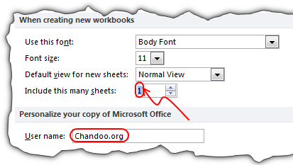
To begin with, I want to have only 1 sheet on my new workbooks as I seldom work with 2 or 3 sheets.
Change the user name
Since many of my workbooks are emailed to clients or uploaded on chandoo.org for you to download, I want to use our website address (chandoo.org) as my username.
Enable Developer Ribbon
After this, I went to customize ribbon and checked the Developer Ribbon box. This ensures that I can see the developer ribbon in Excel so that I can use features like form controls, macros etc.

Note: If you are using Excel 2007, you can find this in Popular tab in Excel Options.
Disable Error Checking Options
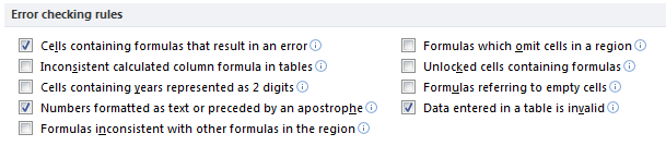
Excel has a friendly feature called as error checking. By default this is enabled and Excel shows warning messages whenever you have made some predefined errors while using Excel. For example, you would get a warning whenever your formulas omit adjacent cells in a region.
While this is useful, I find it annoying as most of the time I know what I am doing. So I disabled almost all of the error checking rules except the ones that I want.
You can do this from Formula options in Excel Options screen.
Tell Excel to take frequent backups of your files
Since the work I do in Excel feeds my family, I want to make sure nothing is lost. Apart from using external back-up applications, I want to use built-in backup features in Excel. You can set these settings from Save tab in Excel options.

Customize Quick Access Toolbar
There are quite a few things in Excel that I use on regular basis. To begin with, I use shapes, alignment tools, text-box, select objects on regular basis. So I add these to my QAT. I will be adding more items to QAT as I use more features on this laptop’s Excel.

Adding Excel to Taskbar
This next is not an Excel tip but Windows tip. Since I use Excel thru-out the day, I just add it to taskbar (by right clicking on Excel in Programs and choosing Pin to task bar.)
What about you?
Those are the bare-minimum customizations I made to my Excel 20101.
What about you? How do you customize your own Excel to make it productive & easy to use. Please share using comments.
More Tips on Customizing Excel
If you want to use Excel productively, then customizing how it behaves is the first step. Here are some handy ideas you can try,
- 10 Tips to make better & boss-proof spreadsheets in Excel
- How to create new ribbons in Excel 2010
- Pin frequently used documents to Excel’s file menu
- 15 Productivity Tips for Excel users (Excel 2003 and above)
- How to add your macros to Quick Access Toolbar
- More Excel Productivity Tips, Keyboard Shortcuts & Mouse Shortcuts
PS: Wish you a happy weekend. We are taking the kids to Safari World today (Friday), for a day of giraffes, monkeys, dolphins, elephants and sun.


13 Responses
I do pretty much the same as Chandoo
I use a Calibri Font at 8 Pt as the default with 1 Page in new worksheets
I add a Print Preview, Print Settings & Quick Print and Record/Stop and VBA buttons to the QAT.
I install the Pup Excel addin.
I also install my own Personal.xlsm file which contains my own library of user Defined Functions and code snipets
I usually install a couple of addins: Name Manager and PUP are almost always on. I usually have query editor and SFE around somewhere as well.
qat: camera tool, watch window, vba editor, query parameters in the
Also in the QAT: record a macro. Did you know that the record button on the both starts and stops recording even when it’s in the QAT?
Also:
Am I the only person who runs the ribbon minimized?
I was ecstatic when I figured out how to minimize the ribbon! I have come to like the ribbon over time, but I still would rather have a maximized workspace for the most part. 95% of what I do can be done with the QAT, shortcuts, or the right-click button on my keyboard.
I do pretty much the same.
I enable the developer ribbon.
I always set the number of sheets to ‘1’ as I never use more than one sheet at a time.
I like to set the default font to Consolas, as it gives a strike through on the zero. I also set the font size to 12 point because my eyesight is not as good these days.
I also add the camera tool to the qat, and move the qat below the ribbon.
I minimise the ribbon and use the alt key to navigate.
Pretty much the same, but I cannot live with some of my addins, most importantly I get the MZTools and the SmartIndenter immediately installed.
It is of course bigger than Excel. I have a list of about 40 items for the whole computer to get it to work the way I want it to. Some Excel 2007 ones follow;
Office>Excel Options>Advanced : Disable edit in cell
Office>Excel Options>Advanced : Disable move after edit cell
Office>Excel Options>Popular : Font Times New Roman
Office>Options>Save : File locations
Office>Excel Options>Advanced – Recent list : Max
Copy Excel.QAT to C:\Documents and Settings\Ken\Local Settings\Application Data\Microsoft\Office [XP]
Office>Excel Options>Popular : Developer On
Office>Excel Options>Trust Center>Trust Center Settings>Macro Settings : Enable macros
Office>Excel Options>Trust Center>Trust Center Settings>Macro Settings : Allow VBA Project access
Re-install ASAP Utilities
Re-install MZ Tools
I also save screen dumps of other Excel Settings
In reply to Dan I always mininimize the ribbon and with about 50 options on the QAT rarely access the ribbon. I also run the Macro record from the QAT but on conclusion of recording the button is re-instated in the status bar (initially turned off). MS – is this a bug?
Clarrification on the record button – the Stop recording button appears on the Status Bar then reverts to “Ready to” Record on the conclusion of recording – not so much a bug but an interface inconsistency.
MZ Tools – all the useful stuff that MS forgot about especially Global Find!
Weird. I haven’t been able to reproduce that.
Ken,
What do you mean the button is reinstated in the status bar? I don’t think I’ve come across any buggish behavior doing this.
Oh. And why have I never heard of MZ tools before? Because that’s pretty awesome.
thanks.
First of all: when I would buy a new computer and already had Office 2010 on the old computer I would export my customizations from the old computer and import them into the new Office package on the new computer. (File – Options – Quick Access Toolbar – Import/Export).
Then set up the templates for a) new workbook b) new worksheet OR copy over form the old machine. So that when you open a new workbook it always has your pre-defined font-settings, print-settings etcetera.
Then copy over your personal Macro workbook.
And then change some general settings which (I believe) cannot be copied over from an older version:
– change user name;
– disable background error checking;
– set the autorecover settings;
– disable “after pressing enter move ..”
– disable “Provide feedback with sound” and “provide feedback with animation” as this slows down your excel when enabled;
– enable the Lotus compatibility – transition navigation keys (Home is really Home then);
– check / change the add-in settings;
– check / change the trustcenter settings.
That’s more or less it.
Regards.
Good post! I actually do most of the things you do. One cool thing I recently discovered is the QAT is “mobile”. You can easily import it into any machine you use so you can keep your QAT consistent across multiple computers. Here’s where I got the info:
http://www.techrepublic.com/blog/msoffice/copy-office-2007-and-2010-quick-access-toolbars/4253
After a too long decade, we just jumped to Office 2010; thank you for these customizing tipps; this will help a lot
From what has been listed, the first and most important thing I do is install ASAP Utilities and OfficeTab.
OfficeTab basically lets me have tabbed browsing with my excel workbooks so that I don’t have a zillion sheets to alt-tab to and from.
ASAP is the most powerful excel add-in I have ever seen and tends to make quite a bit of my older VBA code obsolete.