
Hello folks,
My flight to Sydney has been lengthy but fun. I have reached here on Sunday morning (8AM) and spent most of the day with Danielle’s family. (Danielle is the founder of Plum Solutions. She is the one who invited me to Australia and planned this whole experience for me).
On Monday (30th April), I went exploring the city on foot. I had coffee in the beautiful Queen Victoria Building, attended 1PM church service at the magnificent St. Mary’s cathedral, walked thru Hyde park, went to Sydney central station, took at sneak peek at the new Apple store in down town, got back to my hotel, walked to Opera house to meet up with our readers.
Reader meetup at Sydney
We had 6 people turn up for the meetup. It was fun talking about Excel & our journey with these wonderful folks. Here is a pic (you can see the harbor bridge in background & 8 awesome Excel users in foreground, Click on it to enlarge).

Later in the evening, I took a ferry from circular quay to darling harbor, watching the night lights of downtown Sydney. What a memorable day.
Now, I am getting ready for my first day of Excel training (I am doing a 2 day session with KPMG today & tomorrow), I am feeling excited.
But don’t worry that only KPMG folks are getting their dose of Excel today. I have something for you too. Here is a collection some really interesting Excel links. Click thru to learn more.
Update Data Source of all Pivots
As a data analyst, I am sure you have at least one file that has multiple pivot tables, sourced from different data sets. Now, what do you do when the source data changes? If you are not using Excel Tables, it is a hassle to update all the Pivot data sources to reflect new data. Well, Debra comes to rescue again with a macro that updates all data sources in one shot.
Sending Emails using Excel & Outlook – JP’s take
JP, well known for his Excel & Outlook blog, took a look at our recent Send mails using Excel & Outlook example and rewrote the macro in his style. Check out his code & commentary to understand how you can improve the sendmail macro.
Use Home > Insert to add calculated fields to Pivots
Mike, while making a tour between the snack plate & dip bowl, stumbled on to a very useful feature in the Insert menu on Home ribbon. When you are dealing with Pivots, you can add a calculated field by just using Home > insert. This is a lot faster than doing it from the Pivot table ribbons. I am not sure what dip Mike uses, but I am going to try it too 😉
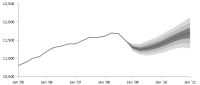 Excel fan charts to show uncertainty in projections
Heard about Excel fan charts? Me neither. But for every Excel charting problem that is as hard as a macadamia nut, there is a Jon Peltier tutorial to show it to you. So in this tutorial, Jon tells us how to create fan charts in Excel to show the uncertainty in projections. Very interesting. And unlike macadamia nuts, this is not going to leave you with broken teeth or bleeding jaws.
Carbon Footprint of Countries [Chart inspiration]
And finally, some chart inspiration. Here is an interactive chart showing the carbon competitiveness index of various countries. Check it out and play with it. And now, go back to Excel and see how you can implement some of those ideas. That will make your Tuesday interesting. 🙂
Got any Excel links that you want to share with us?
I am always looking for new websites and resources to learn Excel & Visualization. So if you came across something that is awesome and want to share it with us, send it to me at chandoo.d @ gmail.com or drop a comment here. Thanks in advance.


24 Responses
I’d suggest simply using the subtotal function and filtering the data using the Win/Loss column. You get the same results and the formula is more comprehensible.
@John
That is one option.
There are times however when you want to see the whole data table or a filtered subset and still want to produce summary reports against an unfiltered field.
Is there a particular reason why you are using a comma and the unary (–) operator for the second array in the SUMPRODUCT formula? It seems to work the same if you were to string the arrays together using the asterisk (*). The advantage is that SUMPRODUCT treats the entire string of arrays as a single array.
@Mathew
Your correct, There is no difference.
I thought it may have been easier to explain this method.
Is there a way to do this on a large set of data? As in ~100,000 rows? When I try I get an error because the formula becomes too long. It says the max length of a formula is 8,192 characters. Excel 2010.
How do I incorporate a specific text within a cell for the second array. For instance, – -(C7:C13=”Apple”)
when I chose a specific text the formula does not work.
@RB
I am not sure what is the issue as if I use the sample data in the post the following work fine
Count:
=SUMPRODUCT(SUBTOTAL(3,OFFSET(C7:C13,ROW(C7:C13)-MIN(ROW(C7:C13)),,1)), –(C7:C13=”L”))
Sum:
=SUMPRODUCT(SUBTOTAL(3,OFFSET(C7:C13,ROW(C7:C13)-MIN(ROW(C7:C13)),,1)),(C7:C13=”L”)*(D7:D13))
You may want to check that there are no leading or trailing spaces in your list of Apples
I should have given a better explanation. Heres my situation. I have a column with cells filled with names like Column 1, Column 2, Pier 1, Pier 2, etc. If the cell just contained Pier and searched for that it works. But because it has other characters in the cell its not recognizing the pier. So how can I extract specific characters of a string of text in this formula?
Hopefully this was a better explanation
Hello-
This formula works pretty well for me except that it slow down excel and prevents some of my macros from working. I was wondering if there was a way to program this in VBA so that excel isn’t always trying to recalculate it. I would like to use a push of a button to get it to run then paste in a cell.
Thanks!
I am trying to sum filtered data in a column, but would want to ignore the negative values in the column. How to go about doing this?
@Akshay
Why not just add a filter to that column to only show the values greater than zero?
The negative values are required for reporting purposes, but their effect on the total is distorting the required output. Please advise.
@Akshay
I’d suggest making a post in the Chandoo.org Forums
http://forum.chandoo.org/
Attach a sample file to simplify the task
I have this working for counting and summing, however, I have a list and for the second array, I need a criteria. That is, I’m looking for b13:b200=”01.??.??” or =left((a1,2) or something like that. These types of criteria matches do not appear to work as I get a blank as a result.
Thanks!
@Bob
As your formula b13:b200=”01.??.??” looks like you are trying to check the first day of the month of the range
What about trying Day(B13:B200)=1
Hai Experts,
i understood this formula well and working fine in MS Excel 2013
but when the same am trying to place in google Spreadsheet it shows error as
“SUMPRODUCT has mismatched range sizes. Expected row count: 1. column count: 1. Actual row count: 2014, column count: 1.” and as a result #VALUE! Appears in cell.
Can anyone please help me how would i get it done in Google Spread sheet
or is there any other formula as a substitute for this.
Thank you very much.
thanks for providing this.. but why does excel keeps on prompting Circular referencing in cell D3?
@Vivek
I don’t know
I just downloaded the file and it is working fine and not showing that error
Goto the Formulas, Calculation Options Tab and check that Calculation is set to Automatic
What version of Excel and Windows are you using ?
I know that this forum is for MS Excel, but I am trying to help someone who is working in Google Sheets. The below formula works in Excel but Google Sheets returns:
“SUMPRODUCT has mismatched range sizes. Expected row count: 1. column count: 1. Actual row count: 39000, column count: 1.” and as a result #VALUE! Appears in cell.
This is the same problem asked by Srichirin above. Does anyone know if there is a formula for Google Sheets that will replicate what MS Excel does?
=SUMPRODUCT(SUBTOTAL(3,OFFSET($C$6:$C$39500,ROW($C$6:$C$39500)-MIN(ROW($C$6:$C$39500)),,1)),- -($C$6:$C$39500=H1),($D$6:$D$39500))
Trying to find a SUMPRODUCT formula that counts the word Closed by date for the last 7 days in a filtered list.
=COUNTIF(M:M,”>”&TODAY()-7) works ok for unfiltered count Column M contains Closure dates (blank if open) and Column L is Status Open or Closed
@ Terry
Please ask the question at the Chandoo.org Forums
https://chandoo.org/forum/
Please attach a sample file to ensure a quicker more accurate answer
I used this formula and worked like a charm! But, now I’ve been requested to use it but adding not one but two criteria in the same formula. For instance the sum I was doing added negative and positive numbers. I’ve been asked to use the exact same formula but adding that only positive numbers were considered… any idea on how to do this?
How exactly do you do sum filtered cells when two criteria are need not just one?
Thank you so much brother literally I have been struggling since morning to get the sum of the filtered category, however, after reading your blog attentively i got my solution, so thanks a lot once again.