
 In excel conditional formatting basics article, we have learned the basics of excel conditional formatting. In this and the next 4 posts, we will learn some more nifty uses of excel conditional formatting.
Let us see how we can highlight top 5 or 10 values in a list using excel as shown aside:
To do this, you need to learn the excel formula – LARGE (more on large formula)
Large formula is used to fetch the nth largest value from a range of numbers. Refer to the above link for easy to understand help on large (and SMALL too)
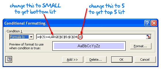
To highlight the top 10 values,
1. Select the range of values and launch conditional formatting dialog.
2. Assuming you have cells in the range c5: c30, In the formula we need to specify a condition that would be true only if a value is more than or equal to the top 10th value in the range c5:c30 – LARGE($C$5:$C$30,10), thus our formula will be, C5>=LARGE($C$5:$C$30,10)
3. Finally specify the formatting you want to apply. When you are done, press ok.
That is all.
If you want to highlight the entire row instead of a cell, you should use $C5 instead of C5. Why so? That is your home work. Here is a little tip on using relative vs. absolute cell references in excel.
To highlight bottom 10 in a list, all you need to do is change the formula from LARGE to SMALL.
Download the example workbook and learn how to highlight top 10 values in a range.
In the next article
We will learn how you can search a spreadsheet full of data using conditional formatting. So stay tuned and if you havent already, join our newsletter.


61 Responses
This is cool trick…..as cool as my do the dew can!!
In case of duplicates in sales values Excel highlights more than 10 values. Is there a way to only get exacly 10?
i know it might not be useful in this example, but i need the same kind of formula for another sheet.
@Andreas: Beautiful question. You can make sure only 10 items are highlighted no matter what by adding a very small running fraction to the numbers. That way you make them unique and then highlight them. You can use a helper column to do this so that your original data stays in tact.
You can checkout more on this technique in our management dashboards posts : http://chandoo.org/wp/management-dashboards-excel
@Chandoo
I was hoping there would be a way. Altough, I looked through these pages but couldn’t find a good example of this method. I am fairly new to Excel, so could you point me in the right direction?
Hi Andreas… You can check this particular post http://chandoo.org/wp/2008/08/27/excel-kpi-dashboard-sort-2/ which is also linked on the earlier page I have told.
We use the technique of adding a very small fraction to numbers to make sure they are always sorted properly.
Also, Oscar, one of our readers sent me this through email: Andreas, try this conditional formatting formula in Chandoos example workbook:
=AND($C5>=LARGE($C$5:$C$34,10),NOT(AND(IF(COUNT(IF($C$5:$C5=LARGE($C$5:$C$34,10),1,””))>1,1,0),$C5=LARGE($C$5:$C$34,10))))
Try this and let me know how it works…
Any one tried the solution given here? It did not work for me as the formula gives me an error.
I have been able to get this to work, but is there a way to list the highlighted items in another location in the spreadsheet in value order? Like a “top ten list” so I don’t have to sort through the whole list to find them?
I have the same question as Lia.
I want to make a Top 5 from SHEETa in a new sheet.
The numbers I want to use are from F11 to F55. But there is also a matching decription
(for example Brand A, Brand B ect.) from N11 to N55.
The problem is that the numbers are NOT unique. Many are/could be the same.
I used this formula to get the top 5 Numbers. I have put these in cells A1 to A5:
=SMALL(SHEETa!F$11:F$55;1) Result:4,0
=SMALL(SHEETa!F$11:F$55;2) Result:4,6
=SMALL(SHEETa!F$11:F$55;3) Result:4,7
=SMALL(SHEETa!F$11:F$55;4) Result:4,7
=SMALL(SHEETa!F$11:F$55;5) Result:4,7
This is correct.
But the trouble starts when I want to show the matching Brand names to these numbers.
I used this formula from B1 to B5
=VLOOKUP(SMALL(SHEETa!F$11:F$55;1);SHEETa!$F$11:$N$55;9;0)
As a result B3 to B5 all show Brand G but is should be 3 different ones.
Is there a sollution to this?
@Lia: you can use the SMALL and LARGE functions to get this work. I am sorry, but I didnt see your comment until Wouter made his entry. You can learn more about these functions here:
http://chandoo.org/excel-formulas/small.html
http://chandoo.org/excel-formulas/large.html
http://chandoo.org/wp/2008/08/13/15-microsoft-excel-formulas/
@Wouter: You can solve this by making the numbers unique. This can be achieved by adding a small unique fraction (like 0.00001 for the first number, 0.00002 for the second etc.) to each of the numbers before sending them to the SMALL(). This can be done with a helper column so that your original values remain intact.
I am sure you can follow this hint and solve the problem. But if you need some more help, feel free to ask.
Changing to small does not give me the bottom 10. What am I doing wrong?
@Glenn… Have you changed the condition from >= to <= ?
I did try <= and it wont highlight the bottom 10.
@Glenn.. strange.. can you share more about your data. May be you can upload the workbook somewhere and link it in a comment. That way one of us can take a look and see if we can help you .
Also, did you check if there is any other conditional formatting on that range of cells with stop-if-true checked ? May be it is preventing you to set the formatting? You can clear conditional formatting by selecting the entire range and pressing clear > formats from ribbon.
Got it… Thanks Guys, it was another conditional formatting preventing this to work.
Hello Chandoo and others.
I have a conditional formatting problem related to SMALL.
I have a column of figures formatted as accounting numbers and includes zero’s. The column is $D$1:$D$24. I want to fomatt the smallest 3 numbers excluding zero’s. I also have the zero’s formatted white to be invisable but I have it ticked off ‘Stop if true’. The formula that works when there are no zeros is
=IF($D10,$D1<=SMALL($B$1:$D$9,3)) but if there are zero’s it fails. Does anyone have the answer. Thankyou
@Les… Welcome to PHD and thanks for asking a question.
I am not sure why you are using IF() in the conditional formatting. You can try the below formula to determine if a given cell is small 3 value excluding zeros…
$D1<=small($D$1:$D$24,3+countif($D$1:$D$24,”0″))
along with that if you set white font color or ;;; custom format code for the zero values, you can hide zeros and highlight bottom 3 values.
Let me know if you face some difficulties.
Hi Chandoo,
It worked beautifully thank you. The IF() was a leftover part of a formula which should have been removed after an attempt at IF(0) trying to eliminate the inclusion of zero’s which failed miserably. You are a very kind person by helping people like me and I love how you do things differently particularly with Charts and think outside the square. Good luck to you sir.
Chandoo,
I am attempting to do the same thing as Les, but the formula is not working as intended.
I have column J2 through J248 that requires conditional formatting, Bottom 10 values not including 0.
When I attempted to edit the formula that you posted for Les to use, I edited it for my column range.
=$J2<=SMALL($J$2:$J$248,10+COUNTIF($J$2:$J$248,”0?))
When I use this, it only highlights the 0’s, in which case I have 53 items highlighted. Instead of highlighting the bottom 10 without the 0’s.
Please help me figure out what I’m doing wrong.
Thank you,
Bryan
Great tip on conditional formatting for top 10 figures!
Question, is there a way of duplicating the conditional formatting for 10 years (or more) worth of data without highlighting each column and reapplying that cond formatting formula for each?
That is, I want the top 10 figures for each year to automatically highlight but right now it seems the only way to do that will be to reapply conditional formatting to each column. Is there a quicker way?
Thanks.
You can use format painter to copy and paste conditional formats from one range to another. It would not more than few clicks to do this. Also, make sure any references in the formulas in the conditional formatting are relative.
HI FRIEND,
I WANT TO KNOW HOW TO USE VB IN EXCEL( IN MACRO).
PLEASE HELP…
I’m using the below conditional formatting formulas to select the Top 3 and Bottom 3 values in a range (excluding Zero). Some of the fields contain percentages (positive/negative) and is conditionally formatting the bottom 4-5 percentage values intead of the bottom 3 percentage values as specified in my formulas.
Conditional Formatting Formulas:
Condition 1: Cell Value Is equal to 0 (No Format Set)
Condition 2: Formula Is =G81>=LARGE(G$79:G$88,3) (Green Font)
Condition 3: Formula Is =G79<=SMALL(G$79:G$88,3+COUNTIF(G$79:G$88,"0")) (Red Font)
The range of values is as follows: (G78:G88)
% MOM
-50.00% (Red Font)
0.00% (Normal Black Font)
-61.54% (Red Font)
-44.44% (Red Font)
-25.00% (Normal Black Font)
-66.67% (Red Font)
-75.00% (Red Font)
-42.86% (Normal Black Font)
66.67% (Green Font)
0.00% (Normal Black Font)
Any idea why this is happening?
Thanks.
Correction to Conditional Formatting Formula:
Condition 2: Formula Is =G79>=LARGE(G$79:G$88,3) (Green Font)
@AWD… you need not add the number of zeros to the small parameter, remember, zeros are greater than negative values. But if your data can often not have any negative values, then you need count of zeros. The condition will depend on how many negative values are there in bottom 3. A simpler alternative could be to just make a helper column and replace zeros with a really large or really small (totally negative) value. This way you can use the count formula as it is.
Dear
i have 20 sheet detial in same format amount is differ…..i have pick 3 smallest on master one sheet.
what is the right formula
@Abdul… use formula =small(masterdata,1) for smallest item, =small(masterdata,2), =small(masterdata,3) for other two.
I have 3 or more columns of server names, each for 1 month.
I need to highlight, the unique servers added or deleted each month from 3 or 4 columns.
some servers are common in all 4 months ( columns also contains their disk size ) but this is adjacent to names.
@Vassajoe
Have a read of http://chandoo.org/wp/2010/07/01/compare-lists-excel-tip/
You may need to work through the columns a pair at a time
Dear Sir
I have one store stock data ,That data contain MRP,System Qty,Phy Qty & Diff Qty.
i need top fifty value in this data. how to get the top fifty value this data
Regards.
V.Sidhu
V.Sidhu
Quickest way is to convert to a Data Table (Insert, Table)
And use selection criteria on the pulldown of the fields you want
Hey Chandoo,
Thanks for the tips on here – they live up to your tag word ‘awesome’! I was wondering if you knew a slick way to highlight the top x% of a range by value rather than number please? E.g we have a range of numbers that total 100 – we want to highlight the top 70% by value, i.e. all the largest numbers that together make up at least 70 (this could be made up by any number of values depending on the range). Does that make sense? The only way I’ve got to do this so far is by using LARGE to effectively sort the list into a seperate one, work out a cumulative total on each value, find the ‘threshold’ point at which that cumulative total crosses 70% and then conditionally format all the numbers that are above the threshold! But there must be an easier way?
I am working on a large array of data. I would like to list top 10 number in column 13 and list down with the values in column 1,2,3,4. in 10 seperate lines. What formula should I use.
@Muhammad
Add a column and use a Rank Formula
arrange as appropriate on Column 13
Then you can use and Index/Match combo to retrieve the data from Column (1 to 4) lookup the highest 10 values from the new Rank Column
You can email me and I can show you on your data if you want.
@huiThank you how can i have your email
@Muhammad
Click on Hui… and at bottom of the page
Chandoo, a fantastic tip on the ‘n’ largest values under conditional formatting but is there a way i can highlight values 6-10 in a different colour? Working with xls 2003 where there are only 3 allowed conditions. I can do them seperate and get values 6 & 7 – but after that i’m stumped!!! Cheers
Thats Superb it helped me a lot 🙂 Thanks Chandoo
I agree with the above chandoo explanation using conditional formatting. I found another example of using top and bottom values for dashboards without conditional formatting.
http://excelprofessor.blogspot.com/2011/10/dashboard-top-5-values-bottom-5-values.html
I have a set of data that I am looking to do Pareto Analysis on.
The sheet has various colums but the key ones are the reason for failure and then the three data inputs which are marked between 1-10. Then there is a final section which adds up the three data entry points to give a risk factor.
I then want to set a table to look for the top 5 (which i know how to do) but then get a fomula which looks at the risk factor matches it to the data table and then looks for the failure mode. Can this be done?
suppose if i have a table with columns on months e.g jan, feb mar etc and under each column is data, is it possible to use conditional formatting and highlight all date related to current month.
Chandoo
How about top 80%?
If I have 13 cells with different data, how do I highlight the top 5 green, bottom 4 red, and the middle 4 yellow??
Hallo,
Can you, please, tell me how can i high light excel rows and column of selected cell in excel 2010 and 2013.
Thanks
sorry i posted here by mistake, it is here http://chandoo.org/wp/2012/07/11/highlight-row-column-of-selected-cell-using-vba/#comment-478551
Hey thanks a lot – needed this for a report today and it nailed it!
I have sales figure of customers each month. However, for some customers I have multiple values within a month too. In this case how do I have publish the list of top customers ?
Example:Company A Product P 2500$
Company A Product Q 3500$
I want the total of Company to be considered and not these 2 separately
I am not getting the rule of top/bottom ten percentage being applied on conditional formatting. Kindly can anyone explain me please???
Hi
I have one small query in addition to this topic. If I have 4 values like
Marks obtained Total Marks
8 10
15 20
12 15
18 30
Now, I learnt from your explanation how to choose the largest values. My question is:
First find the best three marks (as the total marks are different and obviously the % would decide which are best three to choose)
Then those three marks have to sum together (based on the three largest % marks) and then as a whole want to get the % of the sum out of total marks?
BACKGROUND:
As students gave me the assignments 4 and all assignments have different total marks (i,e out of marks like 10, 20, 15, 30). Now I want first to select the best three assignment marks (which is just possible by calculating their % of each as total marks are different). Then sum those three marks and then get the % of them by using the corresponding total marks of each of them.
Your kind reply would highly be acknowledged.
Best regards
Raza
i want to calculate top twenty list out of thousand e.g i have a cell range from A10: A1000 and i want top twenty list the values in this range may b same
regards
plz some help me i want to make a list of top twenty from a range
Dear Sir,
Please find the algorithm below
average of 10sec in Col A (A2:A11) and write the value in D2
average of 10 sec in Col B (B2:B11) and write the value in E2
average of 10 sec in Col C (C2:C11) and write the value in F2
Now this formula in Col G (G2)
=IF(D2-E2 >=2,”RED”,”Green”)
Now this formula in Col H (H2)
=IF(E2-F2>=2″RED”,”Green”)
Now this formula in Col I (I2)
=IF(D2-F2 >=4″RED”,”GREEN”)
Please answer me i want to know how can i do it i will be very thankful to you all the process will keep on doing untill the last value
Hi chandoo,
I want to automate the process of taking top 10 items from different divisions of a pivot table and then deleting the remaining values in a range . Normally I use conditional formatting and delete the remaining values for this but its time consuming as my pivot contains more that 1500 records pls help me on this .
Thanks in advance,
Piradeepa
I have two columns: a list square footage and a list of associated costs. I want to identify the top 5 items on the list with the most square feet with the least cost. Can you assist?
I can highlight top/bottom ten cells but how do you then remove the highlight? If I run a new Top 10 the older highlighted cells stay highlighted even though new ones may be added, so it’s now a Top 17 or whatever.
i have a column of numbers i want the top 5 highlighted but i want each one to have its own color, be it a flag, stoplight or even insert a (1), (2), (3), (4) or a (5) next to the top 5 numbers
@Kenneth
You will need to setup 5 Conditional formats one for each of the 1-5 values
I would use the Large(Range, Number) function
I recommend you ask the question in the Chandoo.org Forums
https://chandoo.org/forum/
Attach a sample file for a more targeted response
I have a pivot table with 8 columns. Each column i am doing top 5 and bottom 5 for driver fuel performance.
I had a lot of 0’s in multiple columns. I went to file, options and changed it so they do not show. I try to create the conditional formatting for bottom 5 and it still highlights all the blank cells that are really 0. how do i get around t his?
You need to use a “formula based” rule as the built-in top / bottom rules can’t recognize such extra conditions. For example, you can say
=SMALL(FILTER(your_column, your_column<>0),5) to findout the 5th smallest value excluding 0 in your_column. You can then apply this logic in CF rules to check if the current cell value is less than or equal to the 5th lowest and highlight.
Thank You Chandoo! I will try that