
The other day, while doing consulting for one of my customers, I had a strange problem. My customer has data for several KPIs and she wants to display average of top 5 values in the dashboard.
- Now, if she wants average of all values, we can use AVERAGE() formula
- if she wants top 5 values to be highlighted, we can use LARGE() formula and CF.
but average of top 5?
I said what any consultant would say. “It is possible”
After thinking for a while, I found the solution by nesting LARGE() formula with AVERAGE() formula. Like this:
=AVERAGE(LARGE(A1:A10,{1,2,3,4,5}))
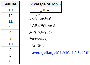
There is no need to press CTRL+SHIFT+Enter after this formula and it works fine.
You can use similar formula to get Average of bottom 5 values like this:
=AVERAGE(SMALL(A1:A10,{1,2,3,4,5}))
Now, your home work:
Ok, here is an interesting twist to this formula. My formula works fine as long as the list has at least 5 values in it. But, lets say the input range (a1:a10) is dynamic. That means, it can grow or shrink.
Now, how would you modify this formula so that it works even when there are less than 5 values ?
Go, figure that out. When you are done, come back here and post a comment.


103 Responses
Thanks for the tip. It’s always interesting to see a new way of solving a problem. Here’s my shot at your homework.
One way to make this work when the range has less than 5 entries (but at least one) is to dynamically create the second parameter for the LARGE function. Instead of always passing {1,2,3,4,5}, this should only be the case when the range is sufficiently large otherwise a shorter array must be passed. So we can replace this by:
IF(ROWS(A1:A10)>5;{1;2;3;4;5};ROW(A1:A10))
If the range doesn’t happen to start on row 1, the row numbering returned by the ROW function must be corrected. So to be correct wherever the range is, the ROW(A1:A10) should be replaced by ROW(A1:A10) – ROW(A1) + 1.
Finally, this needs be an array function (unlike the original).
The whole formula is the following:
=AVERAGE(LARGE(A1:A10,IF(ROWS(A1:A10)>5;{1;2;3;4;5};ROW(A1:A10) – ROW(A1) + 1)))
Hi Martin,
Can u explain why u have used – ROW(A1) + 1))) in the above formula.
Thanks in advance.
Regards,
Gaurang
Imagine if your data is in A5:A14, then this formula becomes,
ROW(A5:A14) – ROW($A$5) + 1
Sorry for the follow-up. Just noticed that I missed a few things while translating the formula from German to English Excel. Of course, the separator for parameters is “,” not “;”. The correct formula is:
=AVERAGE(LARGE(A1:A10,IF(ROWS(A1:A10)>5,{1,2,3,4,5},ROW(A1:A10) – ROW(A1) + 1)))
G’day Chandoo,
How about this:
=AVERAGE(IF(RANK(DataRange,DataRange)<=5,DataRange))
where DataRange is your dynamic range.
Of course you can integrate 'averageif' into this if you're using excel 2007 and 2010, but thought this might be friendlier for those using 2003.
Have an awesome weekend! 🙂
Hy Brook,
I am using your formula for TOP 5 values AVERAGE but I am not gettion exact answer. As per your formula answer is 6.8 but correct answer would be 10.4.
Can you help how can I will get exact answer.
For example my data as mentioned below:-
Data range is A1:A10
10
12
11
9
4
7
10
3
2
0
If I am useing this formula =AVERAGE(LARGE(A1:A10,{1,2,3,4,5})) than my AVERAGE is 10.4
If I am useing your formula =AVERAGE(IF(RANK(A1:A10,A1:A10)<=5,A1:A10)) than my AVERAGE is 6.8
Why so?
My main reason is using using your formula is I want TOP 50 Values AVERAGE in the range of A1:A95000. How can I will get the correct answer
@Jagdish
You can use either
=IFERROR(AVERAGE(LARGE(A:A,{1,2,3,4,5})),AVERAGE(A:A))or
=IFERROR(AVERAGE(LARGE(A:A,ROW(OFFSET(A1,,,5)))),AVERAGE(A:A))The second formula is an Array formula and must be entered with a Ctrl Shift Enter
In the second formula change the 5 to 50 to get the Average of the Top 50
eg:
=IFERROR(AVERAGE(LARGE(A:A,ROW(OFFSET(A1,,,50)))),AVERAGE(A:A))Ctrl Shift Enter@ Hui,
Thanx for your valueable reply.
This Formula is working fine!!!
Thanx once again.
Thanks for the solution.
A small improvement in formula given above for Top 5.
The following formula will work in all versions of excel.
=AVERAGE(IF(COUNT(A:A)<=5,A:A,LARGE(A:A,ROW(OFFSET(A1,,,5))))) Ctrl Shift Enter
Hi Hui,
I was just looking through your formula and was wondering if you could help explain Row(Offset)?
I tried the formula and it works but I’m not sure how it works. I also tried to lock A1 –> $A$1 and the answer came out different but have no idea why. Could you help explain a bit please?
Assumption:
1. Only numeric data in “Values”
2. Maximum number of data rows data are known
In column “B” lets say, put an if logic which checks
if there is a value in “A1”,
if yes than put the same value,
else, if no value put 0 in column “B1″
[ Formula: =IF(A1=””,0,A1) ]
Paste this formula from “B1” through “B10” (assuming 10 max rows of data)
Now use SUM formula on new data column “B1:B10”
[ Formula: =SUM(LARGE(B1:B10,{1,2,3,4,5})) ]
Also, use COUNT formula to count number of rows on original data column “A1:A10”
[ Formula: =COUNT(A1:A10) ]
Finally we divide SUM with the COUNT to get AVERAGE on a dynamic list
[ Formula: = SUM(LARGE(B1:B10,{1,2,3,4,5}))/COUNT(A1:A10) ]
Is this too long for a solution. 🙂 Looking for more ideas.
BTW … thanks Chandoo, I have been a regular reader and great work.
I have learnt many things from the blog, keep up the good work.
Cheers, Parveen
Create MyDynamicRange equal to
=Sheet1!$A$1:INDEX(Sheet1!$A:$A,COUNTA(Sheet1!$A:$A))
Then enter this
=AVERAGE(LARGE(MyDynamicRange,IF(ROWS(MyDynamicRange)>5,{1,2,3,4,5},ROW(MyDynamicRange))))
with Control+Shift+Enter.
How about these:
=AVERAGE(IF(COUNT(A:A)<5,OFFSET(A1,0,0,COUNTA(A:A),1),LARGE(OFFSET(A1,0,0,COUNTA(A:A),1),{1,2,3,4,5})))
or with a named range where "myRange" = "=OFFSET($A$1,0,0,COUNTA($A:$A),1)"
=AVERAGE(IF(COUNT(A:A)<5,myRange,LARGE(myRange,{1,2,3,4,5})))
Hello Chandoo…
Here’s my shortest guess :
= AVERAGE( LARGE( A1:A10 , OFFSET( E3:E7, 0,0, MIN(5, COUNTA( A1:A10 ) ), 1 ) ) )
and press CTRL+SHIFT+ENTER
the helper column E3:E7 contains 1, 2, 3, 4 ,5.
By the way I’ve found a website translating every Excel function into several languages
http://dolf.trieschnigg.nl/excel/excel.html
If anyone figure how to enter a {1,2,3,4,5} array into offset instead of using the helper column…
Cyril
Chandoo,
Here’s how I would do it.
.
=AVERAGE(LARGE(dr,ROW(OFFSET(dr,,,MIN(5,ROWS(dr))))))
.
with Control+Shift+Enter, and “dr” is the dynamic range.
No IF() functions needed, which Dick may be interested in knowing 🙂
Regards,
Daniel Ferry
excelhero.com
I used the following formula and it worked fine
=IF(COUNT(B2:B14)<5,AVERAGE(B2:B14),AVERAGE(LARGE(B2:B14,{1,2,3,4,5})))
Some interesting answers in the comments above. A number of formulas are being used that I have never used before….very interesting. Could someone explain the meaning of the use of {} in the LARGE formula. This is something new to me. Thanks.
I would use {=AVERAGE(IF(LEN(A1:A10)>0,LARGE(A1:A10,{1,2,3,4,5})))} (array entered!)
Have a nice weekend!
CC
@Abbas Sura –
{} is how you specify an array of constants. Some of Excel’s functions, such as LARGE, SMALL, AND, and OR (and some others), can work with an array of values without requiring the entire formula to be Array-Entered.
.
In Chandoo’s LARGE formula for the blog entry, the {1,2,3,4,5} array compels the formula to pull out the first largest value in the range, then the second, then the third, then the fourth, and then the fifth, and to average them together for the result. The problem is that if you give the LARGE function this directive and there is no fifth largest value (because there is only four values in your range), the LARGE function will produce and error.
.
Using arrays in formulas can be very potent, as is taking it one step further and making the entire formula an “Array Formula”, as many of the examples above demonstrate, including mine.
.
@CC –
Your formula does not work for me.
.
Regards,
Daniel Ferry
excelhero.com
What about:
=IFERROR(AVERAGE(LARGE(A:A,{1,2,3,4,5})),AVERAGE(A:A))
A non-volatile, non-array (in that it doesn’t require CSE) dynamic range option:
=SUMPRODUCT(LARGE(A1:INDEX(A:A,MATCH(9.99999999999999E+307,A:A)),ROW(A1:INDEX(A:A,(MIN(5,MATCH(9.99999999999999E+307,A:A)))))))/MIN(5,MATCH(9.99999999999999E+307,A:A))
Can be consolidated further by naming last row & dynamic range
lr=MATCH(9.99999999999999E+307,$A:$A)
dr =$A$1:INDEX($A:$A,lr)
To:
=SUMPRODUCT(LARGE(dr,ROW(A1:INDEX(A:A,(MIN(5,lr))))))/MIN(5,lr)
I created a named range “Data” and used offset (=OFFSET(Sheet1!$A$2,0,0,COUNTA(Sheet1!$A$2:$A$200),1)). I then added the name “Data” into the original formula in place of the array (=AVERAGE(LARGE(Data,{1,2,3,4,5}))).
I created a named range “Data” and used “=OFFSET(Sheet1!$A$2,0,0,COUNTA(Sheet1!$A$2:$A$200),1)” in the refers to field. I then replaced the array in the original formulas with “Data”. “=AVERAGE(SMALL(Data,{1,2,3,4,5}))”
@Shel Price –
Your formula will not work when there is less than five entries in the dynamic range. Chandoo’s objective was to find a formula that would work for five or more (like his does and like yours does), but ALSO for less than five entries.
Regards,
Daniel Ferry
excelhero.com
What about:
=IFERROR(AVERAGE(LARGE(A:A,{1,2,3,4,5})),AVERAGE(A:A))
That provides for less than 5, and the top 5 no matter where they are in the column.
Yeah, I saw that after I posted. Tested for more rather than less.
My dodgy tuppence worth (CSE):
IFERROR(AVERAGE(LARGE($A:$A,MID(ROW(INDIRECT(“1:”&MIN(COUNT($A:$A),5))),1,1))),””)
(Error in case there are no values).
MyRange equal to.
=$A$1:INDEX($A:$A,MATCH(9.99E+307,$A:$A))
Formula to get the average
=CHOOSE((COUNT(MyRange)>5)+1,AVERAGE(MyRange),AVERAGE(LARGE(MyRange,{1,2,3,4,5})))
Regards
Dear Chandoo,
With all due apologies to my Hero Daniel Ferry here is a solution from a lesser mortal
With a dynamic range named Data
=IF(COUNT(Data)<5,SUM(Data)/COUNT(Data),AVERAGE(LARGE(Data,{1,2,3,4,5})))
Daniel Ferry, you are not only a hero but an Excel Picasso as well, I really enjoy your Excel Hero blog. But a question please IF i may.
When and IF ever have you used IF. All the solutions that you propose without IF are truly elegant.
Chandoo Thanks for a most inspiring web site
Cheer
Kanti
@Kanti –
Here is a quote from a comment I left one of my readers recently regarding the IF() function:
.
“I am not philosophically opposed to the IF() function. It’s just that I feel it is used too much and often when there are better choices. However, when it comes to throwing an #N/A to force data points to hide themselves on a chart, I think that IF() is an excellent choice. For some reason, Excel is able to conditionally (with the IF() function) output an #N/A at lightning speed.”
.
This comment was from my celtic muse blog entry:
http://www.excelhero.com/blog/2010/05/excel-animated-chart-2.html
.
Kanti, I’ve found over the years that if I force myself to look for solutions that do not rely on the IF() function, two things happen:
1.) I discover angles of attack on a problem that would never have occurred to me otherwise and hence interesting solutions that are sometimes elegant and sometimes not.
2.) The exercise makes me a better formula crafter in all situations.
.
Regards,
Daniel Ferry
excelhero.com
Hi guys,
Hope that this solution can help.
The formula I use is just a slight modification of the formula shown in the article.
Let data_range = cell range that contains the numbers
Key in (or copy and paste) the formula below in a cell
=Average(large(data_range,row(indirect(“1:”&min(5,count(data_range))))))
and press control+shift+enter
In this case, if the range contains more than 5 figures, only the average of largest 5 figures will return; if less than 5 figures, the average of those figures will return.
Please let me know how do you think about it.
Thanks and best regards,
Eliel Lew
=IFERROR(AVERAGE(LARGE(–DynamicRange–;{1;2;3;4;5}));AVERAGE(–DynamicRange–))
if the dynamic range is named NamedRange then:
=IFERROR(AVERAGE(LARGE(NamedRange ;{1;2;3;4;5}));AVERAGE(NamedRange))
David Ferry,
OFFSET is a volatile function and is always recalculated at each recalculation. This can slow down large excel sheets considerably. Should volatile functions be avoided??
@Oscar –
While OFFSET is volatile, it is extremely fast, and with it some amazingly creative solutions can be found. I routinely use it on large projects with many thousands of formulas with no problem. The advice to look for nonvolatile solutions is sound, but it should not be absolute. ROW() is also listed as volatile, but it has NEVER adversely affected one of my projects.
With OFFSET and ROW in particular, it is well worth exploring their use. Every circumstance is unique, but I would never shy away from either of these.
By the way, my name is Daniel (but I do have a brother named David – though I don’t think he knows what Excel is ;))
Regards,
Daniel Ferry
excelhero.com
Excellent contributions by everyone. Thank you so much for the creativity and ideas you have shown here.
One observation in general.
When the list has less than 5 values, Average of top 5 is nothing but average. So the simplest way to write this formula can be,
=AVERAGE(IF(COUNT(A1:A10)<6,A1:A10,LARGE(A1:A10,{1,2,3,4,5})))
But then again, you have shown so much more variety in your answers. Thank you. 🙂
Just what I was looking for, thanks!
Hi
This is my solution
=IF(COUNTA(A:A)<5,AVERAGE(A:A),AVERAGE(LARGE(OFFSET(A1,0,0,COUNTA(A:A),1),{1,2,3,4,5})))
Thanks for the amazing site.
Row() is not volatile. It is wrongly listed as volatile
@Chandoo –
That may be the simplest, but I think Brook’s formula (comment #3) is the best.
=AVERAGE(IF(RANK(dr,dr)<=5,dr))
where "dr" is the data range.
.
Elegant. I even liked how Brook used the IF() function. Cudos Brook!
.
Regards,
Daniel Ferry
excelhero.com
I agree that this is a great formula, but after testing it, there is one flaw in that if values tie for 5th place or lower, it will skew the average. This, as opposed to the large formula which will explicitly pull back 5 values.
Great use of a function I’ve never seen though. Really elegant formula.
Dear Mr Daniel please read my quetion and answerit i am really in a Need and i ind your answe very usefull
@Tahir or Saleem ?
Two different names and same question, what goes?
You need to setup a column of values for each Range
ie
A2 =1/3600/24
A3 = 2*A$2
A4 = (Row()-1)*A$2
etc
Then use an =Averageifs function to retrieve your average scores
If you post the question at the Chandoo.org Forums
http://forum.chandoo.org/
Please attach a file and you will get a more targeted response
@Brook – comment #3
Asking for your Solution with Excel 2007
Can you explain, how to write the formula AVERAGEIF (using Excel 2007)?
Chandoo, Thanks for your very inspiring excel site.
Thanks and best regards,
aldus
thanks for the tip it made me perfect in our exam
thank you very much!!!!!!!!!!!!!!!!!!!!!!!!!!!!!!!!…………….,,,,<<<<<<<<
CHANDOO I TRIED THIS FORMULA BUT AM NOT GETTING THE ANSWER I MENTIONED
=AVERAGE{LARGE{A1:A10,(1,2,3,4,5)}} .AM NOT GETTING THE ANSWER.
B1=AVERAGE(LARGE(adi,{1,2,3,4,5})) will work definately…
adi is the range for whole column.
you can select range by selecting the whole column A1 to A65536
using ctrl up and down and after selection plz mention adi in
top left cell address area.
Its working completely fine for me
let me know if anyone needs help on this 🙂
I hope chandoo will be proud of me..
Hi – being a bit lazy by not defining a dynamic range name – but this formula does the job (i think) =AVERAGE(LARGE(A:A,ROW(INDIRECT(“1:”&IF(COUNT(A:A)
Dear All,
This is the one valued Trick on excel.
I have a question where I want calculate AVERAGE with with TOP 50 values where my data range is A1:A15000.
How can I will calculate I don’t want to type mannually 1 to 50. Inside of LARGE Function values. Is there any way how can I will caluculate?
=IFERROR(AVERAGE(LARGE(A:A,{1,2,3,4,5})),AVERAGE(A:A))
Thanx in Advanced!!!
@Jagdish
Try the following Array formula
=IFERROR(AVERAGE(LARGE(A:A,ROW(OFFSET(A1,,,50)))),AVERAGE(A:A))It has to be entered with Ctrl Shift Enter
Change the Value 5 to 50 to suit
This is the formula I made up which includes two added components:
1. average based on a condition
2. weighted average if over 4 values.
=CEILING(IF(COUNTIF($C$10:$C$60,$B66)>4,AVERAGE(SMALL(IF($C$10:$C$60=$B66,$R$10:$R$60),$W$5) * $W$6, SMALL(IF($C$10:$C$60=$B66,$R$10:$R$60), $X$5) * $X$6, SMALL(IF($C$10:$C$60=$B66,$R$10:$R$60), $Y$5) * $Y$6, SMALL(IF($C$10:$C$60=$B66,$R$10:$R$60), $Z$5) * $Z$6) * 4, AVERAGE(IF($C$10:$C$60=$B66, $R$10:$R$60))), 5)
Now if someone could improve my formula so that the weighted averages worked with 4 or less entries, I would be impressed (and grateful)!
A few questions… what about calculating the standard deviation of the top five… is it just a simple? Also, what happens if there are three items tied for fifth place? One three items tied for second place?
What if I wanted not the top 5, but rather the top 50% of the data?
Hi
I would like to take the top 5 average for a number of scores in specific columns. What would be the formula say if the columns were F8, I8, M8, O8, R8,T8, W8 for example?
Thanks
=AVERAGE(LARGE(($F$8,$I$8,$M$8,$O$8,$R$8,$T$8,$W$8),ROW(OFFSET($A$1,,,5,1)))) Ctrl+Shift+Enter
or
=AVERAGE(LARGE(F8:W8,ROW(OFFSET($A$1,,,5,1)))) Ctrl+Shift+Enter
or
=AVERAGE(LARGE(myRng,ROW(OFFSET($A$1,,,5,1)))) Ctrl+Shift+Enter
Where myRng is a Named Formula
myRng =Sheet1!$F$8,Sheet1!$I$8,Sheet1!$M$8,Sheet1!$O$8,Sheet1!$R$8,Sheet1!$T$8,Sheet1!$W$8
I am a college student and I wanted to create an excel sheet so I could easily input my quiz grades and figure out my quiz average. My professor drops our lowest 2 quizes out of 7 but before I had all of my quiz grades I still wanted to know what my average was so I used the above formula with a slight modification so that it will average regardless of the number of values i currently have entered and will give me my average of only my top 5 scores. This is my modified formula:
=IF(COUNTA(B2:B11)>4,AVERAGE(LARGE(B2:B11,{1,2,3,4,5})),AVERAGE(B2:B11))
I simply used
=AVERAGE(LARGE(arrr,1),LARGE(arrr,2),LARGE(arrr,3),LARGE(arrr,4),LARGE(arrr,5))
where arrr= array
=AVERAGE(LARGE(arrr,{1,2,3,4,5}))
i want to count the numbers that means i have 40 to 100 numbers i want to count how many numbers are there between 50 to 59 manually i can count 10 or may be 6 numbers so to calculate using excel what shall i do
@Yassin
Try using the Countifs() function
It will be something like: =Countifs(A1:A100, ” GT 50″, A1:A100, ” LT 59″)
Change the range and GT LT etc as appropriate
GT = Greater than
LT = Less Than
So what would this look like if you wanted to calculate the average of the highest 5% (or 10%) of the numbers. I have a data range that has 4000 values and i want the average to the top 200 (or 400) items?
Any thoughts??
Assuming your values are in column A, the formula can be modified as
=AVERAGE(LARGE(A:A,ROW(OFFSET(A1,,,CEILING(COUNT(A:A)*5%,1))))) Ctrl Shift Enter
for average of top 5% Values.
Greetings Im trying to create a formula that measures the avg high and low of several different arguments for instance
=AVERAGE(LARGE(E3:E14,E19:E30,E51:E62,E35:E46,E67:E78,E97:E108,E126:E137,E156:E167,E185:E196,E214:E225,E230:E241,E246:E257,{1,2,3})) is there anyway for this to work.
Hi Chandoo,
That was a great tip man, thanks a lot for posting the formula!
Nadav
Hi Chandoo,Iran hui,
hi am working one similar kind of data,
Data:
Each line of Transaction has
Date, Hour, Job processed, Average processing(dynamic), CPU Util
10-04-2016,04:01:00PM,3700,5500,90%
Average processing value is dynamic that i should calculate when the CPU util is more than or equal to 90% and i should only consider last 4 Job procesed transactions + current tranaction with CPU util greater or equal to 90 %. Please suggest some way to do this in excel.
Hi everyone
I have done an experiment and sensor gives me reading after every 1ms (millisecond). There are thousands of row ( 3 – 993434) I want to do something in excel to reduce the number of rows e:g average) or through some calculation in a new colum so that I will be able to get the values for every 1sec
Means it will give me 1 value for one second and 60 values for 1mint
@Tahir or Saleem ?
Two different names and same question, what goes?
You need to setup a column of values for each Range
ie
A2 =1/3600/24
A3 =(Row()-1)*A$2
A4 =(Row()-1)*A$2
etc
Then use an =Averageifs function to retrieve your average scores
If you post the question at the Chandoo.org Forums
http://forum.chandoo.org/
Please attach a file and you will get a more targeted response
Hi everyone
I have done an experiment and sensor gives me reading after every 1ms (millisecond). There are thousands of row ( 3 – 993434) I want to do something in excel to reduce the number of rows e:g average) or through some calculation in a new colum so that I will be able to get the values for every 1sec
Means it will give me 1 value for one second and 60 values for 1mint
For example I have a data set in colum A with 1000000 number of rows I am trying to reduce the data set by averaging every 1500 rows in this data frame, How can i do that. I am very new to Excel
@Saleem
Same Question, now different question, what is going on ?
You need to setup a column of values for each Range
ie
A2 =1
A3 =(Row()-2)*1500
A4 =(Row()-2)*1500
etc
Then use an =Average with an offset to retrieve the various ranges defined by the row numbers above
If you post the question at the Chandoo.org Forums
http://forum.chandoo.org/
Please attach a file and you will get a more targeted response
Hi Hui thankx, I am sorry for two Name ist my first and last Name i haved tried to post the question and have not found the question and i again post it with my second Name
hi hui can i have you time on s kype to get the expert advice
@Saleem
I don’t do Excel Consulting
You have asked this question about 10 times now,
Every time I have asked you to:
“If you post the question at the Chandoo.org Forums
http://forum.chandoo.org/
Please attach a file and you will get a more targeted response”
Thanks all for ingenious solutions!
Can anyone solve this,
If l am having an average value of 59% for 5 Days and want to bring it down on 50% on 6th Day for which the value should be 5% of 6th day but l have to do this on manual basis but require a formula to do it so e.g
1-Jul 2-Jul 3-Jul 4-Jul 5-Jul 6-Jul AVG %
59% 59% 59% 59% 59% 5% 50%
Thanks Steven for your comment and welcome to Chandoo.org
Assuming your original data is in A1:E1 and target average is in A2, write below formula.
=A2*(count(A1:E1)+1) – sum(A1:E1)
Thanks Chandoo: but guess what l am still having the same answer and the answer is 50%
Sorry it’s 59% instated of having 5%
Not sure I understand the problem. Adjust the A2 value to whatever target average you want and the formula will give the answer.
@Steven
Looking at your data above and assuming the dates are in Row 1, Chandoo’s formula should be:
F2 should be: =G2*(count(A2:E2)+1) – sum(A2:E2)
where G2 has the Target Value 50%
it should be like this
=5*A2-SUM(B1:E1)
A2>Target Value
B1:E1>last 4 days data (and should be dynamic to be updated everyday )
Thanks Chandoo: Your a Jew bro… it help after understanding…..
Dear all i want to know that the average of top 100 values in colum A starting from A2 to A101 and put the value in B2: after it is finished with avg of top 100 values then it moves automatically to next avg of A102 to A 202 and put the value in B2
is it possible that i can do it in excel
Let me rephrase the question
Average of A2:A101 in B2
Average of A102:A201 in B3
… and so on.
i.e., average of 100 numbers at a time in consecutive rows.
The formula in B2 is :
=IF((ROW()-2)<CEILING(COUNT(A:A)/100,1),AVERAGE(OFFSET($A$2,100*(ROW()-2),0,100)),"")
the same can be copied and pasted in subsequent rows till the point the result is not blank.
Hi @Arun N. This falls right in line with something I’m trying to accomplish. Rather than subsequent rows, is it possible to do this by % ? For example, I want to average the first largest 25% within the list of values. Then the next 25% of the largest. And so on.
@Shane
Can you please ask the question at the Chandoo.org Forums
http://chandoo.org/forum/
Please attach a sample file to get a more targeted response
@Hui Ok thanks. I have done so.
I want to attach one file can i do it ?
=IFERROR(SUMIF(values,”>=”&LARGE(values,5))/COUNTIF(values,”>=”&LARGE(values,5)),AVERAGE(values))
Note: I defined the range as “values” for dynamicity.
=IF(COUNT(A1:A10)>5,AVERAGE(LARGE(A1:A10,{1,2,3,4,5})),AVERAGE(LARGE(A1:INDEX(A1:A10,COUNT(A1:A10)),ROW(A1:INDEX(A1:A10,COUNT(A1:A10))))))
¡Muy practico! Contundentes criterios. Manten este nivel es un articulo genial. Tengo que leer màs blogs como este.
Saludos
=IF(COUNT(A1:A10)<5,AVERAGE(A1:A10),AVERAGE(LARGE(A1:A10,{1,2,3,4,5})))
If there are fewer than five cells containing values, excel will simply average all the values. Remember that excel automatically ignores blank cells when calculating averages within a given range.
Please Tell me, if i’m fill the value in First column & Row the
reflectet to next column & Row. And if First value in addition &
Subtraction then reflected to next column also.
A B
12+5 1200 then ok
if (1200-100) refleted (1100)
both are one column reflected
=averageif(A:A,”>=”&large(A:A,5))
This says compute the average of the cells in column A if they are >= the 5th largest value in the column
This code fails the prompt that it needs to be able to calculate the values if there are less than 5 inputs. Hardcoding the nth integer when there aren’t that many values returns an error.
=AVERAGE(IFERROR(LARGE(A1:A3,{1,2,3,4,5}),””))
or for whole column:
=AVERAGE(IFERROR(LARGE(A:A,{1,2,3,4,5}),””))
=SUMIF(H3:H12,”>=”&LARGE(H3:H12,IF(COUNTA(H3:H12)<5,COUNTA(H3:H12),5)))/IF(COUNTA(H3:H12)<5,COUNTA(H3:H12),5)
=IFERROR(
LET(range,A1:A20,
filter,FILTER(A1:A20,A1:A20″”),
sort,SORT(filter,,-1),
rows,ROWS(sort),
topvalus,IF(rows>4,TAKE(sort,5),sort),
AVERAGE(topvalus)
)
,”NO Data”)