
Here is a 2011 new year gift to all our readers – a free 2011 calendar template.
(a little secret: just change the year in worksheet “Full” from 2011 to 2012 to get the next year’s calendar. It works all the way up to year 9999)
You can add notes to individual dates or complete month using the excel template very easily. There are 6 different calendar templates in the download file,
- 4 Yearly Calendar Templates with different color schemes.
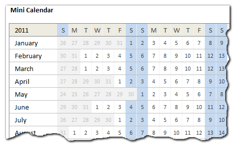
- 1 Mini Calendar
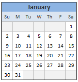
- 1 Monthly Calendar (prints in 12 pages)
![Free 2011 Calendar - Download and Print Year 2011 Calendar today - Excel Spreadsheet Template for Yearly Calendar [2011]](https://img.chandoo.org/c/2011-calendar-template-download-free.png)
Download 2011 Excel Calendar Template
Download the Printable 2011 Calendar – in PDF format
Download the 2011 Calendar Spreadsheet – Excel 2007+ | Excel 2003
More Calendars: Year 2010 Excel Calendar | Year 2009 Excel Calendar
How this Calendar works?
Read on if you are curious to know how the formulas are cooked in this calendar…,
- The cell D3 in worksheet Full has the year of calendar. I named this cell as year.
- All the formulas for the calendar are written in the worksheet mini.
- For this year’s calendar, I took inspiration from Daniel’s Live Calendar example (Recommended reading for formula enthusiasts).
- The first step to create a calendar is to generate a sequence of numbers 1 thru 42 (because calendar grid has 42 cells – 7 days per week x 6 weeks max, per month). I used a combination of INDIRECT, OFFSET and COLUMN to get this. The formula is
=COLUMN(OFFSET(INDIRECT("$A$1"),0,0,1,42))-1. I mapped this formula todaysAndWksnamed range. - Next step is to find the first date of each month using a simple date formula like
=date(year,month,1). This formula is mapped to named range –DateOfFirst - For given month, the calendar is nothing but
=daysAndWks + DateOfFirst - WEEKDAY(DateOfFirst,2). This formula is mapped to named range – calendar.
 Once the mini calendar is ready, I just created 12 named ranges m1_, m2_,…, m12_ corresponding to each of the 12 months.
- Then, I used the same in individual calendar worksheets along with INDEX formulas to fetch the dates.
- Finally, I formatted the calendars nicely. Design of this calendar is similar to that of 2010 calendar & 2009 calendar templates.
Go ahead and enjoy the download. The file is unlocked. So poke around the formulas and named ranges. Learn some Excel.
More Downloads: Download Free Excel Templates
Techniques used: INDEX | OFFSET| INDIRECT | Array Formulas | Using Date & Time in Excel


32 Responses
Thanks! The only thing that I would add is no. of the week.
Chandoo,
impressive !!! a beautiful and useful file indeed.
Also, please check http://www.todoexcel.com/calendario-laboral/ (in Spanish). They have a great calendar as well, with the ability to list festivities and holidays, and then they are displayed in different colors on the calendar. It had proven to be a great tool as well.
Rgds.
Martin
Brilliant Sir. Marvelous.
Even as someone who is more than competent at Excel, this never ceases to amaze me.
cheers,
Amazing !
Thanks a lot for your great work and for having allowed access to the formulas.
All the best!
Shalom from Israel
This is great timing. I have been working on a spreadsheet to track some information and this fits the bill perfectly. I have made a few adjustments to make it work for Academic Years (July through following June) and voilà!
Thank you so much!
David
Great work!
Also just a quick question … Would it be possible to upload data from excel into a web page.
Say, for example, if I do a personal journal diary entry in a similar template, would it be technically possible to sync that into my google calendar – the additional challenge being to sign in to my google id.
Regards,
Renjith M Das
Thanks Chandoo. I’ll put this on the Ribbon which I use in office with a button to bring up this calendar.
Merry Christmas to you and family.
Thanks chandoo, but can you explain how to “add notes to individual dates or complete month using the excel template” ??
Merry Christmas to you and family.
by the way I was looking for some thing similar from quite a while, I want to use it like a table planer most of us use in our offices where we take notes in the date box for daily works etc. to keep note of important chores for next day.
I hope I explained correctly I mean if I click cell ” 5 January” the notes taken for that date should appear in the “notes” column. then If click some other date it should change the coulmn content to that date …
Thanks
This is fantastic just what I needed. I’m a complete excel novice this is just ace. Can you tell me if I can use it to work out the dates of placements ie I want to be able to tell when my students should complete a 100 day placement so say if they start on the 6th jan is there a way I can put a formula in to work out when the 100 days is up.
many thanks
Very Nice indeed – thank you….
Just amzing
Fantastic! By far the most useful calendar I’ve found to date! Thank you.
Thanks for the Calendar. I have downloaded it and I have changed it for 2012.
Is there a way to work out the date of the nth working day of the month? For example, 4th working day of March12, which is 6th March 12. Thanks.
Regards
Premalatha
@Premalatha
=WORKDAY.INTL(“1/3/2012”,4)-1
or
=WORKDAY.INTL(“29/2/2012”,4)
or in older versions of Excel
=WORKDAY(“1/3/2012”,4)-1
or
=WORKDAY(“29/2/2012”,4)
Thanks for the reply. I did try that, but I am using it inside so many other calculations in which I have a variable “month” and I would like this Workday.intl to work taking “month” as input.
got it.
WORKDAY.INTL(Month-DAY(Month)+1,Days,)! 🙂
(“month” was Today() and so was never the 1/month/year.) It is working now. Thank you.
forgot to mention, those “Month” and Days were my locally defined names for other formulae and are not the functions available in Excel. But “Day” is excel function I used to estimate the number of days from the start of the month.
Fantastic! I want to design a 2013 calendar using kukuruku/chicken/turkey/ostrich as illustration. Your assistance would be highly appreciated and applauded.
Thanks.
hello, fantastic calendar, let me ask you a question, is it possible to adapt it so that i can have two years?
How do I merge my excel file with all my calendar information for the academic year 2012-2013 with your template?
Nice calendar but I want to use it like a table planer so i can take notes in the date box for daily works. to keep note of important chores for next day. Is this possible?