

There are beautiful, powerful & awesome charting examples all around us. Today, I want to show you how we can harness the power of Excel to create Analytical Charts.
Analytical What?!?
To be frank, I do not know what to call these charts, so I choose the term Analytical Charts. But this is what I have in mind (see below) when I say Analytical charts:
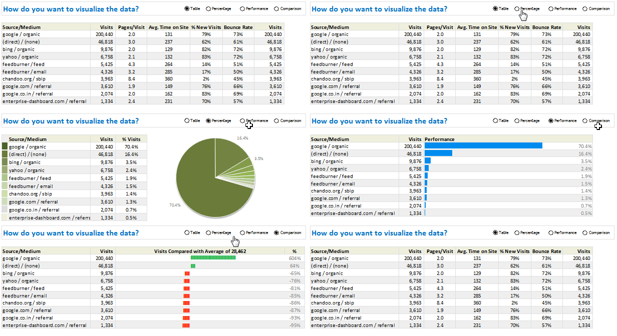
A chart is analytical chart,
- If it is interactive
- It it can answer different questions by re-structuring same data differently
What is the inspiration for Analytical Charts?
Google Analytics. I use Google Analytics, a web-app that tells me about the visitors and traffic flowing in to my site. It gathers millions of data points every day and presents all this information in rich, easy to read views. One of the powerful features of Google Analytics is that, you can tell it to show the same information in different views so that you can answer different questions.
On top of every report in Google Analytics, we have these buttons:
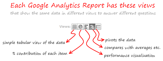
When you click the button, the report is instantly restructured to answer a different question.
So how to make such charts in Excel?
The basic technique behind this is similar to the one we discussed in show one chart from many article. Since, It would be 1800 word long if I describe the process, I decided to make a short video (18 minutes) explaining how the charts are constructed. Watch the video tutorial below:
Excel Analytical Charts – Video Tutorial:
The Process for creating Analytical Charts:
- Make individual views of the data in different cell ranges.
- Name each range uniquely, like chtRng1 for tabular view and chtRng2 for percentage comparison view etc.
- Insert radio buttons (option buttons) from developer ribbon > forms, one each for a different view.
- Now, link all the radio buttons to same cell. That way, when select a view the linked cell would show corresponding number.
- Create a named range called chtSel and point it to a CHOOSE formula that would select the corresponding named range defined in (2)
- Now, select any few cells, press CTRL+C and paste them as a picture link. (tutorial on picture links).
- Select the picture link, go to formula bar and type =chtSel
- That is all. Now, you have made an analytical chart that makes your boss love you.
Download Excel Analytical Chart Example Workbook
Click here to download the example workbook. This should work in Excel 2007 or above.
Do you use Analytical Charts?
As I mention in the video, I find the “views” option in Google Analytics quite useful. It hides answers for questions that are not yet asked. But with just a click, I could visualize information in a different way.
What about you? Do you find analytical charts useful or as clutter? How would you implement them? Please share your ideas and techniques using comments.


42 Responses to “Prevent Duplicate Data Entry using Cell Validations”
Hi Chandoo, I need you help in the following problem.
I'm trying to get a direccion from a found result. With this dirreccion I will want the before cell value. For example, If result of a find is 38 localized in cell $C$2, I need to get previus value (cell $B$2 ), maybe Andrés.
Do you know some way to do that?
Thank you for you help.
Hi Chandoo
Thanks for this. One thing though: In my pre-2007 version of Excel, the COUNTIF function doesn't recognise a semicolon (;), but requires a comma.
Is the semicolon an Excel 2007 thing?
Jair... I am not sure I understand what you want. what do you mean by Dirreccion?
@Lincoln: I am sorry, often I forget that I am using European version of excel where the delimiter is ; instead of ,. I have corrected the formula now.
Thanks for this nice tip, i used to do a find all after filling every new items which was cumbersome.
Do you know a way to extend this validation search to other tabs/sheets ?
Thanks for you attention. I'm trying to get of value continue from a found value. Let me show a example:
Name Years
John 35
Maria 28
Teresa 32
If I search the max years, the result is 35, but I need that result to be John. Do you know how I can do it?
@Subbu.. you can easily extend the validation to other sheets by pasting the data validations. See the latest article here: http://chandoo.org/wp/2009/10/28/copy-data-validations/
@Jair.. you can use the large() or small() formulas to do this. for eg. =index(A1:A3,large(B1:B3,1)) will get you the name of the person with highest "years". More help here: http://chandoo.org/excel-formulas/large.html
Hi, I don't know if I'm using bad the formula or its performance is diferent for my Office version. Large() formula return the value in the cell, in my example 35. The index() formula use a range, row and column. I'm using the large() as number of row, and it is bad because into the range don't have row 35. This is my perception. What do you think?
Hi, I going to prove, with this solution by JLD http://jldexcelsp.blogspot.com/2008/07/extraer-direccion-de-celda-en-matriz.html
Hello,
I am trying to attempt data validation in Excel Mobile, but the DV tool isnt available. I want to prevent duplicates is all, any advice on acheiving this in Excel Mobile? Thanks..
@Jair... my french aint that good. it starts at "merci" and ends at "beau coup".
Anyhow, you need to merge the large with vlookup to do this. I am not sure if you have solved the problem. Otherwise let me know with details and I can write the formula in comments.
@Chad... I have never used excel mobile, so I have no idea. May be they have not implemented data validations in excel mobile.
Any excel mobile users out there?
Hi Chandoo, the proposed solution by JlD is interesting. He created a macro to get values when the matrix is not one dimensional, how on my problem. This fuction for me.
I would like to share you my work, how can I upload?
@Jair.. sorry for such a delayed reply.. you can upload the files to skydrive and link them here. Or you can email them to me at chandoo.d @ gmail.com and I will upload them somewhere. But it could take forever if you email files to me as I am a bit lazy.
[...] Day 31: Advanced Data Validation Tricks in Excel – Part 2 [...]
Hi,
Can you help me in Microstrategy?
Br,
Moin
really wonderful article. I feel it is implementing Primary Key concept into spreadsheets.
Hi article on data validation. Excel is a very versatile platform to work with and we use it for all kinds of data tabulation. In fact this must have been the most rudimentary data management tools I must have worked with and knowing such tips only adds functuionality to our user experience. Great article. looking forawrd to read more.
Hi Chandoo,
Thanks for such a nice idea.
I tried copy paste the data into the validated area, but the pop-up msg (warning msg) doesn't came. Is it something that we need to update the data manually each time,.
Do we have any option where we can bulk upload the number and it throws a warning message that the data already exits and do we want to continue with this ?
Please do reply me.
Thank you.
Regards,
Vasanth.
It was really useful chandoo...thanks a lot...
Tried this in excel 2010 and it did not work?
Could the newer excel have changed that much?
@Leo
It works fine in Excel 2010
The formula used above =COUNTIF($B$4:$B$11,B4)<=1
only applies to the range B4:B11
Did you adjust the range to your data?
This page helped me accurately to find solution of my question. thanx
we want to prevent duplicate entries in three columns combined, using data validation, i.e. say, column A has first name and Column B has middle name, Column C has last name. the first name can be duplicate, middle name can be duplicate, last name can be duplicate, but not all three at the same time.
I want to prevent duplicate entries in three columns combine, using data validation, i.e. say, column A has first name and Column B has middle name, Column C has last name. the first name can be duplicate, middle name can be duplicate, last name can be duplicate, but not all three at the same time.
Hi, I've tried above validation method to prevent duplicate value from entering into the cells. It's work, when user key in the data into the selected range. However, it's not working when user copy-&-paste the info into the same range.
Please advice. Thanks.
Hi Chandoo,
Does it work in Excel 2007?
Please Reply
thanks chandoo........
it does not work when data is copy pasted...any solution for this??
hi i m shaloo and i want to know in excel if i write duplicate no.then it says or show about we are write duplicate no.
Hi Chandoo
I've tried using this with a Named Range, which is actually a column in a Table as DV wont accept a table reference, and it wont work.
Also tried using Offset to specify the Named Range, but that wont work either.
Is it possible to use Named Ranges with DV?
Thanks
Kris
I have tried the above formula on a table column. The Error box does not pop up, there is only the small ! next to the cell with the duplicate. The column I am working with is formulas that produce a date. Is the reason it doesn't work that the cells contain formulas rather than data?
The formula works but only if I enter data in cell above it. So for example, if I have "123" in B11 it does not allow me to enter "123" in B10, B9, B8, etc. But I can still enter "123" in B12. Please help! 🙂
Great tip.. thanks a lot
I have 21 years of experience working as data entry assistant. I constantly read several blogs to keep myself up-to-date with the advances in data entry profession. I really enjoyed this blog post. From my several years of experience, I agree with you 100% when you say, “ We all know that data validation is a very useful feature in Excel. You can use data validation to create a drop-down list in a cell and limit the values user can enter. ”
Keep blogging. I will come here again.
--data entry assistant
Hi,
This is really very helpful.
Thank you
how can i assign two validation on a single cell
one is for list validation (means the data should be from that range)
second i want to prevent them from repetition
how can i do this ?
P7 to P506 have GR# which are for list
i want to prevent C column to not to repeat and should be from the P column
@Junaid
Can you please post the question in the Chandoo.org Forums
http://forum.chandoo.org/
You have to register to be able to post questions
Please attach a file so that a specific answer can be delivered.
i made an account but there is no option available to post questions ??
where can i ??
@Jubaid
Goto http://forum.chandoo.org/
Goto Ask an Excel Question
Post New thread
Type your question
Attach a file
Please attach a file so that a specific answer can be delivered.
friend can any one tell me the formula
exname location qty
gaurav 1 1
rofan 2 5
sandeep 3 6
gaurav 4 3
rofan 5 4
sandeep 6 8
gaurav 7 9
If this is a data.
if i want a formula by which if i type gaurav then all the location and qty should be shown in a new page.
i had 5,00,000 sku so if i punch one name i can get the entire details
@Gaurav
Can you please post the question at the Chandoo.org Forums
http://forum.chandoo.org/
Please attach a sample file for a quicker more targeted response
IF(ISERROR(INDEX($B$3:$C$9,SMALL(IF($B$3:$B$9=$B$12,ROW($B$3:$B$9)-ROW($C$2)),ROW(A1:C1)),2)),"",INDEX($B$3:$C$9,SMALL(IF($B$3:$B$9=$B$12,ROW($B$3:$B$9)-ROW($C$2)),ROW(A1:C1)),2))
please explain
YOUR COUNTIF FORMULA IS REALLY HELPFUL AND WORKS. I TRIED SEVERAL SITES BUT THEIR FORMULA DOES NOT WORK. ONLY YOU HAVE GIVEN A RIGHT FORMULA!
THANK YOU!!!!!