
The other day, I got a text message (SMS) from one of our readers. It read,
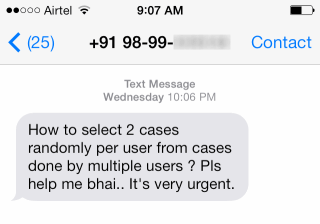
So today, let us learn a very easy trick to select random sample from your data.
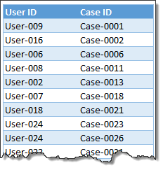
Lets take a look at the data
Since the text message has no actual data, I made up this.
Now, if you just want to select any 10 (or x number of) random items from this list, then your job would very simple.
- Shuffle (or randomly arrange) this list
- Just pick first 10 items
But our problem is to get 2 random samples per user.
Selecting random samples from data
Follow below steps.
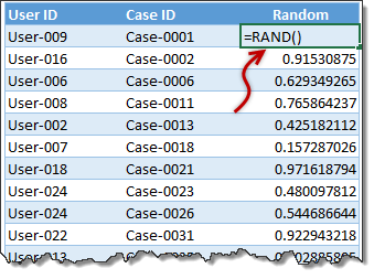
- Add an extra column and fill it with =RAND() formula. This generates random fraction between 0 and 1.
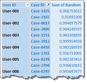
- Create a pivot table from this data (tutorial: How to create a pivot table?)
- Add User ID & Case ID as Row labels and Random as value field.

- Click on the filter icon on Case ID column, choose Value filter > Top 10
- Filter for top 2 random values. (related: Filter top 10 values in pivot tables – how to?)

- Adjust report layout (Table layout, no sub-totals, no grand totals)

- Done!
To see new samples
Just select any cell in the pivot table, press ALT+F5. Your pivot table will be refreshed and you get new samples.
That is just easy and awesome!
Download Example Workbook
Click here to download the example file. Refresh the pivot table (ALT+F5) to see fresh samples.
Do you sample your data?
Drawing samples, running experiments, analyzing results are life breath for many businesses. As business data is growing, these analytical skills are becoming important.
How do you draw samples? What techniques you use when analyzing the data? Please share your stories, experiences & tips using comments.
A sample of our awesome collection of Excel tips
Here is a tiny sample of our awesome Excel tips. Don’t hold back, take them all, and more.
- Introduction to Pivot Tables
- How to shuffle a list of values in Excel
- How to shuffle a list using Formulas
- How to generate a random date, phone number
- Introduction to Excel’s random functions
- Case study: Generating housie (bingo) number cards using Excel
- Game: Simulating Deal or No Deal game in Excel


18 Responses to “How to select a random sample from all your data [trick]”
Great tip and very easy to apply, thank you very much! How do you make the text of the cell screen blur (besides - 99?
After adding "RAND" column, we could add "rank per group" column. Then by filtering for 1 and 2, we will get random 2 rows per user.
=SUMPRODUCT(($A$2:$A$20=A2)*($C$2:$C$20>C2))+1
Is it possible for anybody to create this in VBA with a button or with the help of macro ? It shpuld give randomly 2 cases per user with one click. Please help me if you can.
First time I have tried to download a sample spreadsheet for some time - I am missing something? It is downloading as a zip file even though the shortcut shows it as http://img.chandoo.org/pivot/random-samples-thru-pivot-tables.xlsx
How do I turn the zip file back into something useful?
@Robert
Save the file instead of Opening the file
Then in Explorer rename it to random-samples-thru-pivot-tables.xlsx
Then Open from Explorer or Excel
[…] How to select a random sample from all your data […]
thanks for the trick
Hey Chandoo!
We emailed last week. I've been trying to download your dashboards, no luck! I just set up paypal, but doesn't seem to be working yet, although I've done all they've asked.
Is there anyway we can do this billing directly??
I would like to get this dashboards going asap and have spent two days waiting for paypal !
Regards,
Blaine
PS- Nice looking family you have!
Is there a way of selecting the number of cases to be extracted based on the value in a cell, so that the user can decide how few or many random elements they want selected?
Hi Chandoo,
I enjoyed your tutorial on using random numbers. However, when I tried to open the sample spreadsheet your provided, I learned that the alt+F5 function does not work the same way in my Excel software (Excel for Mac 2011). Would it be possible for you to provide such examples for Mac users as well? I believe that the Windows and Mac versions are largely similar in terms of functionality, but there are a few differences that sometimes make it necessary to describe the differences.
Separately, I am interested in subscribing to the Excel and VBA courses and want to know if the course supports Excel for Mac. Can you confirm?
Any help would be greatly appreciated.
Feel free to respond to me via my email address.
Thanks!
Simple yer highly effective tip.
If i need to have different sample size for each user what should i use.
Thanks in advance.
Regards
Ram
I have excel data with Team Lead name and their team members processed request per day basis. I want to pull 10% of each individual data to do Quality check. How to pull these 10% of each individuals?
Example; 1 TL has 20 team members out of which one member proceseed 100 request I need to pull 10% of 100 request(10 request).. Like this i need to pull all individuals details..
Note: Total number of request processed by teams will be around 6500 request approx
I also have the same question can you please help
@Simi
Can you please ask the question at the Chandoo.org Forums
https://chandoo.org/forum/
Please attach a sample file so we can fully understand your requirements
HI Hui,
I have posted the same with "Random 10% Data Sample in each category actioned by assignee for Quality check"
Regards
@Vishwanath
You may wish to have a look at a solution here:
https://chandoo.org/forum/threads/random-10-data-sample-in-each-category-actioned-by-assignee-for-quality-check.36728/
Can we get 10% of sampling using this trick
Great article, Chandoo! I wanted to extend my appreciation for sharing this easy trick on selecting random samples from data in Excel. The step-by-step process you provided, including the use of the RAND() formula and pivot table, is incredibly valuable. It's fantastic to see how you've made sampling easier and more efficient for data analysis. Thank you for your insightful tips and tricks!