This is a guest post by Faseeh, one of the Excel Ninja’s at our forum.
Triangular plot…! What is it?
Recently, a Chandoo.org forum member asked this,
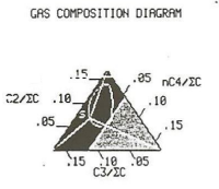
I want to be able to make a graph that, in some aspects, looks like below, but I have no idea how to do it at all.
After seeing it, I said to myself in Barney Stinson’s tone, ‘Challenge Accepted!‘
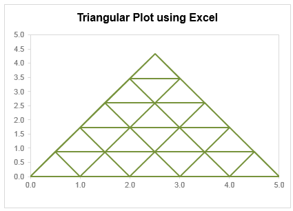
The final plot is like this:

Making triangular plot in Excel – Tutorial
The first step to create such a chart starts from a manual drawing of how your chart will be looking like; at least you need to mark some important connecting points that will make smaller triangles.
The trick in this chart is simply to locate points in all three sides of the triangle and connect them in a way that results in smaller triangle. Here is a step by step approach to make this chart:
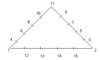
- Make a rough sketch of the triangle. Divide each side of the triangle roughly into the number of segments that you want, each side with equal number of segments (in this case 05 segments). And give each of them a number including corners of the triangle

- Now we can split this chart into three types of lines, horizontal, tilted towards right, tilted toward left.

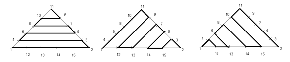
- For each of these lines we need to join certain points and when we combine these lines into a single series we will get our desired chart. So let’s list down the points in each line.
Horizontal Lines (L1): Point 01, 02, 03, 04, 06, 05, 07, 08, 10, 09, 11.
Right Lines (L2): Point 01, 11, 09, 12, 13, 07, 05, 14, 15, 03, 02
Left Lines (L3): Point 02, 11, 10, 15, 14, 08, 06, 13, 12, 04, 01 - Now we need to setup a table where the coordinates of these points are listed in tabular order, like this:

This can be done by using trigonometric ratio of sine and cosine, by representing each point in terms of Polar Coordinates [ These coordinates represent each point in terms of a distance “R” and an angle represented by Greek alphabet Theta (q), Line 01 makes an angle of 0° from X-Axis, Line 02 of 60° and Line 03 of 120° from +ive X- Axis, these details can be simply skipped if you don’t like math 😉 ]
Avoiding the details of trigonometry you can simply use following two formulas to get these values…For Value of X (Ordinate) you can use the following formula:
=IF(O6=”H”,N6*COS(RADIANS(Q6)),IF(O6=”L”,N6*COS(RADIANS(Q6)),$D$5+N6*COS(RADIANS(Q6))))For Y (Abscissa) you can use following:
=IF(O6=”H”,N6*SIN(RADIANS(Q6)),IF(O6=”L”,N6*SIN(RADIANS(Q6)),N6*SIN(RADIANS(Q6)))) - Once this Lookup Table is created we need to create another table where we list points in accordance to the Lines that we have already created. We will use VLOOKUP () to fetch the corresponding coordinate through this formula and we will do this for all the three Lines. The VLOOKUP() simply looks for the point in the left most column of the first table and bring the corresponding values from the 3rd and 4th column to form the point in second table.
- When we are done with bringing the coordinates of all of these points we just need to plot a Scatter Chart. Now use a XY scatter chart to plot the data. You need to add only one series, actually there are three types of lines but we can accommodate them in just one series. When they overlap, they will give smaller triangles in result.
Download Triangular Plot workbook
Click here to download the chart. Examine the formulas & chart series to understand how this is made.
Added by Chandoo
Do you make such complex charts for your work?
I will be honest. I never had to make a triangle plot. But then, I never had to make Ratatouille either. That doesn’t make me appreciate both of them any less. I think this chart shows fantastic technique. It also proves that Excel is highly flexible if you know which bolt to turn and which screw to tighten.
What about you? Do you make such complex charts or visual analysis for your work? What is the most challenging chart you have worked on? Please share using comments.
Shape up your Chart skills – Charts + Shapes
If your job involves making charts in all shapes and sizes, then you are in luck. Check out these tutorials to learn how to bend Excel charting rules to get any shape you want:
- Simulating a pendulum movement using Excel charts
- Wall hygrometric physics – modeling wall thickness in Excel chart
- Stars and lights using Excel Charts, VBA & animation
- Mustache shaped chart to measure your stash
- Spoke chart | 5 star chart
- Making various country flags using Excel charts
Thank you Faseeh
Many thanks to Faseeh for sharing this tutorial with all of us. I really enjoyed this and learned a few tricks from it.
If you like this chart, say thanks to Faseeh using comments.


27 Responses to “Sum of Values Between 2 Dates [Excel Formulas]”
I would apply a filter and use function subtotal, with option 9. This way you can see multiple views based on the filter.
hey Chandoo, the solutions you proposed are very efficient, but if I wanted to be fancy I would do it this way .. the references are as your example workbook.
=SUM(INDIRECT("C"&(MATCH(F5,B5:B95)+4)):INDIRECT("C"&(MATCH(F6,B5:B95)+4)))
I like things simple:
=SUMIF(B5:B95,">="&F5,C5:C95)-SUMIF(B5:B95,">"&F6,C5:C95)
use something like: =SUM(OFFSET(B1,0,0,DATEDIF(A1,D1,"d")))
and have D1 be the date that I want to sum to.
In Excel 2003 (and earlier) I'd use an array formula to calculate either with nested if statements (as shown here) or with AND.
{=SUM(IF(B5:B95>F5,IF(B5:B95<F6,C5:C95,0),0))}
Note that I truly made this for BETWEEN the dates, not including the dates
I turned the data set into a table named Dailies.
I named the two limits StartDate and EndDate.
And used an array formula:
{=SUM((Dailies[Date]>=StartDate)*(Dailies[Date]<=EndDate)*Dailies[Sales])}
If I would still be using the old Excel I would do it as follows:
SUMIF($B$5:$B$95,"<="&H6,$C$5:$C$95)-SUMIF($B$5:$B$95,"<"&H5,$C$5:$C$95)
Works as simple as it is.
Regards
=sum(index(c:c,match(startdate,c:c,1)+1):index(c:c,match(enddate,c:c,1))
=sum(index(c:c,match(startdate,b:b,1)+1):index(c:c,match(enddate,b:b,1))
Great examples and thanks to Chandoo. You have simplified my work.
Hi! great tips I have found in your page, have you seen this
http://runakay.blogspot.com/2011/10/searching-in-multiple-excel-tabs.html
[...] I'm not sure I understand your question fully, but have a look at this: Sum of Values Between 2 Dates [Excel Formulas] | Chandoo.org - Learn Microsoft Excel Online [...]
Thank you! Thank you! Thank you!
=SUMIF(A2:A11;">="&B13;B2:B11)-SUMIF(A2:A11;"<"&A11;B2:B11)
awesome... thank yoo Chandoo!
which is most efficient and fast, if all are efficient ?
Thank you for this formula, I've just spent ages trying to find something to work on my data, I knew it would be possible! Don't care if others think there are easier/other ways to do it, you explained it so I understood it and could apply it to what I was doing so I'm happy!
The above said example is awesome for calculating values between dates,
can you pls let know how to calculate sale values if we have 10 sales boys for
ex: 1,rama
2,krishna
3,ashwin
4,naga
5,suresh
how much rama sale value between 1/jan/2015 to 10/jun/15
how much krishna sale value between 10/jan/2015 to 15/july/2015
i think you understood can you pls let me know the formula for how to calculate the sale between diffrent sale man sale value from master data file
Thanks,
Nagaraju
Hi
I have a list of people's names in column A, I have a list of dates in column B which records the dates they have been off sick, in column C I have either 1 if it is a full sick day or 0.5 if it is a half day.
What I would like to do is to add up the number of dates a specific person has been off within two dates.
For example, I want to look at my list of names and to find Joe Bloggs (column A), then add up all his sick days (column C). The start date will be in cell E1 and the end date will be in F1.
If this possible using SUMIFS?
List of names are in range A2:A100
List of dates in B2:B100
List of sick days (either 0.5 or 1 in C2:C100
The start date is in cell E2
The end date is in cell F2
Your help would be greatly appreciated.
Yes, with the help of SUMIFS you can have the solution.
Note: you need have an extra col. D2 where you will input Name of the person.
=SUMIFS(C2:C100,A2:A100,D2,C2:C100,">="&E2,C2:C100,"<"&F2)
Col. A Col. B Col. C Col.D Col. E Col. F
Name Date Sales
ABC 28-Jun-11 1 MNO 28-Jun-11 25-Sep-11
XYZ 29-Jun-11 0.5
MNO 30-Jun-11 1
PQR 1-Jul-11 1
Typo ERROR / Correction in formula:
Yes, with the help of SUMIFS you can have the solution.
Note: you need have an extra col. D2 where you will input Name of the person.
=SUMIFS(C2:C100,A2:A100,D2,B2:B100,">="&E2,B2:B100,"<"&F2)
Hi
I have a list of people's names in column A, I have a list of dates in column B which records the dates they have been off sick, in column C I have either 1 if it is a full sick day or 0.5 if it is a half day.
What I would like to do is to add up the number of dates a specific person has been off within two dates.
For example, I want to look at my list of names and to find Joe Bloggs (column A), then add up all his sick days (column C). The start date will be in cell E1 and the end date will be in F1.
If this possible using SUMIFS?
List of names are in range A2:A100
List of dates in B2:B100
List of sick days (either 0.5 or 1 in C2:C100
The start date is in cell E2
The end date is in cell F2
Your help would be greatly appreciated.
Viv
@Viv
Can you please post the question in the Chandoo.org Forums
http://forum.chandoo.org/
Please attach a file so that a specific answer can be delivered.
Thanks for this - it solved the problem that I was having. However can someone please explain to me why the "" needs to be around >= and <= as well as why we need to add & in order for the formula to work? Thanks in advance!
This formula works perfectly as well. Any ideas?: =SUM(INDEX(C5:C95,MATCH(H5,B5:B95,1)):INDEX(C5:C95,MATCH(H6,B5:B95,1)))
ikkeman had posted the same thing.
I am trying to sum total a range of cells between date ranges ie column n has $ amounts column d has the transaction dates ie 1/3/2015 or 25/3/2015 or 25/4/2015 column b has the text saying drp or distribution - reinv
In another cell I am trying to sum or total (in column n) with the value of a range of different dates (column d) that contain different text (column b) ie cell n48 is 50, n65 is 85, n165 is 36
with the dates ie cell d48 is 1/3/2015, d65 is 25/3/2015 and d165 is 25/4/2015
with different text that says drp or distribution - reinv ie cell b48 is drp, b65 is distribution - reinv, b165 is drp
If I wanted to sum the amounts between 1/3/2015 to 31/3/2015 with drp then the total would be 50. Also if I wanted to sum the amounts between 1/4/2015 to 30/4/2015 with drp the sum total would be 36 If I wanted to sum the amounts between 1/3/2015 to 31/3/2015 with drp and distribution - reinv the sum would be 115
What would the formula be for these different questions
hope you can help, it has been driving me nuts and cant work it out