
 Today we will learn about Pivot Table Report Filters.
We all know that Pivot Tables help us analyze and report massive amount of data in little time. Excel has several useful pivot table features to help us make all sorts of reports and charts.
Report Filters are one such thing.
How do Report Filters help you?
Let us say, you are an analyst at ACME Inc., that has 3 products – Fastcar, Rapidzoo and Superglue. You have 4 salespersons – Joseph, Lawrence, Maria & Matt. You operate in 3 regions – West, North and Middle.
Now, you are given the data for all sales from Jan 2007 to July 2009 and your boss asks you, “I need a report on sales by product and salesperson in each region”.
This is where a Report filter would help you.
You can put Salesperson in Row label area, Product in Column area, net sales in value field area and region in report filter area of the pivot table. Then, you get a report like this:
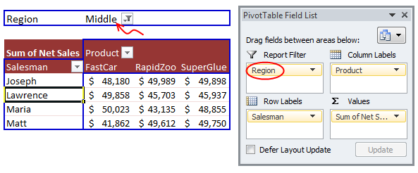
You can immediately switch the report filter to other regions (or a combination of them) to produce the region-wise reports.
Generating Multiple Reports from One Pivot Table:
Using Report Filters, we can quickly generate multiple pivot reports. For this,
1) Click anywhere inside pivot table, and go to Options ribbon.
2) From here, click on little down arrow next to options, choose “Show Report Filter Pages”.
3) Select the filter field for which you want multiple pages.
4) Done! Excel produces multiple worksheets, one each for a report filter setting.
See this demo:
Few more tips on using Report Filters
Add Multiple Report Filters
You can add more than one report filter to a pivot table. This is a very useful way to slice and dice your data when you have lots of columns (dimensions). For eg., you could add report filters on Month, Region & Product.
Show Report Filters in rows or columns
From Pivot Table Options, you can set how Excel should layout the report filters. This setting is available in Layout & Format Tab.
 Select More than one value for Report Filter
By default, Excel allows you to specify only one value per filter. But you can over-ride this by using the “Select multiple items” check-box in report filter.
Download Report Filters Demo Workbook
I have made a demo workbook showing how you can generate multiple reports from same pivot table. Go ahead and download the workbook.
Click here to download Report Filter Demo Workbook.
How do you use Report Filters
I often use Report filters to generate reports for a specific time-window or product group for my small business. I generally do this while analyzing sales or something. For eg. I would make a pivot chart with sales data and add a trend-line to it. Then I would change the report filter to instantly understand the trend for a different product. I like the power report filters give me in situations like this.
What about you? Have you used Report Filters before? In what situations do you find report filters help-ful. Please share your experience & tips using comments.
More Articles on Pivot Tables
If you would like learn more about Pivot Tables, go thru these articles:


32 Responses to “What are Pivot Table Report Filters and How to use them?”
Hi, I'm relatively new to this wonderful site--just signed up for the newsletter yesterday, and the timing of this topic couldn't be more perfect for me! I've been using the "Show Report Filter Pages" option in Excel for a while now (as described in the "Generating Multiple Reports from One Pivot Table" section). It's a great tool, but what would be even greater is if a similar function exists to create multiple charts from one pivot chart! Does anyone know if this feature exists in Excel? Thanks!
Thanks! I like pivot table, too. I am heavy user of pivot on the 2003 version, more so than the 2007 version which I'm currently using. Personally, I find 2007 pivot a bit less intuitive and user friendly than 2003, but just by a little bit. Not a lot.
My challeng of using pivot is that sometime (may be I'm to blame) I can't get pivot to display the way I want it to be. Sometimes it is the count not sum, sometimes it's other things.
Because I'm not using pivot lately with 2007, I wonder if it still explode the file size with every new pivot table created? Most of us deal with thousands of lines and we'll be tasked with creating multiple pivot tables for others to read, or use the data from the pivot tables created for other things.
And I have difficulties to make columns with sub-columns. For instance, I would be asked to display in the form of product families by sales.
Row = Salesman
Columns = Major Product Family A with 3 products and Major Product Family B with 4 products and so on.
And boss doesn't want to have any product families filtered out. He wants to see the whole product lines.
Thank you, Chandoo! I am new to Excel and was working on a Pivot Table. Your tip on report filters has really helped.
@Excelophile: Welcome to Chandoo.org & thanks for joining our newsletter.
Unfortunately, you cannot create multiple pivot charts from one. You need to just manually copy / paste the pivot charts or use a macro to do that.
@Fred: You are welcome. I think the file size grows as you add pivot tables to it. You can set some options to clear pivot cache, but still Excel needs to calculate and store the results.
For sub-columns problem, you can use grouping option in Pivot Tables. It is quite powerful.
@Satya... You are welcome 🙂
[...] Last week, we have learned what Pivot Table Report Filters are & how to use them. [...]
this is very good and use ful for every one
Sadly it seems that this option isn't available for pivot tables from OLAP data cubes
[...] for multiple salespersons. Since you want to show the report by one person at a time, you used report filters in pivot tables to display this. But you find that switching between regions is a pain using the [...]
hi Chandoo,
Your blog is awesome!
I'm currently working on Report Filters and found a limitation to it that it cannot function like Data Filters in Excel. I need to limit pull-down choices to non-zero results. Hope you could help me. Thanks,
Ros
Hi,
I just found your website and let me congratulate you! All this information is very powerful and it will make a great difference in the way I do my work. Im looking forward to browsing more and learning. Thanks!
Chandoo,
Great blog! I'm having the same problem that Ros is having with the limitation on multiple filters. Is it possible to have Pivot Filters be additive in Excel 2007? I.e. If I had 3 Filters (Country, State/Province, City) and I select USA for country, can the second filter only have relevant states listed in it and not states/provinces from other countries? Thanks!
Hi Cory,
Did you get the response for your query, because even i have posted similar question. If yes, please share the same, it would be really great help.
I created a couple of report filters and made some output files from the pivot table by using these report filters.
The problem is my main data source is updated every week and I have to refresh my pivot table which is fine, i am just worried that if there is a shift in the columns and rows due to new additions in the pivot table the output files can not be just refreshed and have to be created again.
Is there any option in which the output files created from the report filters will be automatically updated even when there is shift in the cells? please help
I like this "Report Filter"... They are very useful. What I am currently looking for is: How do I create a report filter via VBA in Excel 2007? I have been looking out for this for a while but did not get anything satisfactory. Any support out here?
Master 😀 Chandoo,
your website is one of the best things I found in the net. Great job and keep it up!
I have one issue with this subject. Imagine you have 2 report filters in one Pivot table ( Region and City ) and some values for this data. You want to create separate sheet for every City, but only for filtered Region. Example: I only want to create each city sheet for North Region.
I'm asking if there is any way to do this with Show pages option?
Again - thanks for huge input in this site.
Cheers
Chandoo,
Can the Slicers option of 2010 be forced in Excel 2007?
Eg, if I have a list of Sales persons and regions, if I select one sales person, I only want to see his regions in the next report filter.
Thanks,
Hi,
Is there anyway that you can 'Show report filter pages' but for column labels.
Thanks
[...] to manipulate. Next begins your love affair with pivot tables to slice and dice the data. (See: What’s a pivot table and how do you use [...]
Is there anyway where i can copy all the available option from pivot filter to specific range? I want to show them in listbox rather than using pivot filter directly and then pass the selected values from listbox to pivot filter directly.
I am able to pass values from listbox to pivot filter but not able to copy value or choices from pivot filter to range
Sir,
When i use Report Filter then all records show in row labels for filter more.
Is there any option available that When i use Report Filter and select one record then show only those records in row labels which fall only under that selection record, for filter more instead of all records in a sheet.
thanks.
I use this function in a report regularly for a similar purpose - so show individual reports by staff members. Where I'm stuck is when I add new staff members. Is there a way to add a new person and have excel just create a tab for the new person (rather than regenerating all of the individual pages)?
I wanted to check about "report filter" and your page gives very clear explanation. Great job. Many thanks.
[…] to manipulate. Next begins your love affair with pivot tables to slice and dice the data. (See: What’s a pivot table and how do you use […]
First, let me say that this website is outstanding. So much excellent information! I do however have a question regarding Pivot Tables. I haven't found an answer yet so hoping someone can help. Is it possible to hidden items in a pivot table but still include them in the grand total? I am currently using Excel 2010. Basically, I have a PT that includes sales for both associates and mangers. I would like the managers totals to be included in the grand total but do not want their names to be seen in the PT. I have numerous PT's that I manually hide the managers on a daily basis. It has become both time consuming and leaves room for errors. Any ideas??
Can we group values of a variable in the Report Filter? For example if I have countries in report filter and I want to group them like say Eastern, Western etc.. can I do that? I know this grouping can be done in Row/Column Labels. But not sure if this can be done in Report Filter too.
Generating Multiple Reports from One Pivot Table is limited to my data and I do not know how to solve it
I have data for each day entered as a number.
then i want to create 12 tabs for each month.
Just changing the date to custom setting mm does not work also not pin pivot tables. When you do this and then do Generating Multiple Reports from One Pivot Table. Excel starts to create a tab for each DAY. How can I convert this?
thank you!
Hi,
I would like to know if its possible to make some kind of filter on the "grand Total" by line on a pivot table.
So basically the grand total would be an additional filter
Thanks in advance for the help
Hi Everyone,
I am in a need of some help in pivot table.. I have multiple report filters, For ex : Country, State, City... If I select 1 particular country, I need to see only those states that are existing in that country instead of all states of all countries, followed by relevant cities existing under selected "state" instead of all cities of all states / countries.
Thanks in advance...Will be waiting for your response.
@Mahesh
I'd suggest asking the question at the Chandoo.org Forums
http://forum.chandoo.org/
Attach a sample file will allow us to give a specific answer
Hi Hui,
My query is similar to the one asked by cory on Jan 4th. I tried to ask the question in the forum you mentioned but I am not getting the option to share the question.
Kindly provide your help in this regards.
Thanks.
@Mahesh
You have to Register to be able to post questions
Then goto: http://chandoo.org/forum/
Select the appropriate Forum, eg: Ask an Excel Question
Then select the "Post new thread" button near the centre top of the screen
very helpful. thanks!