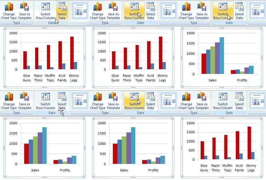
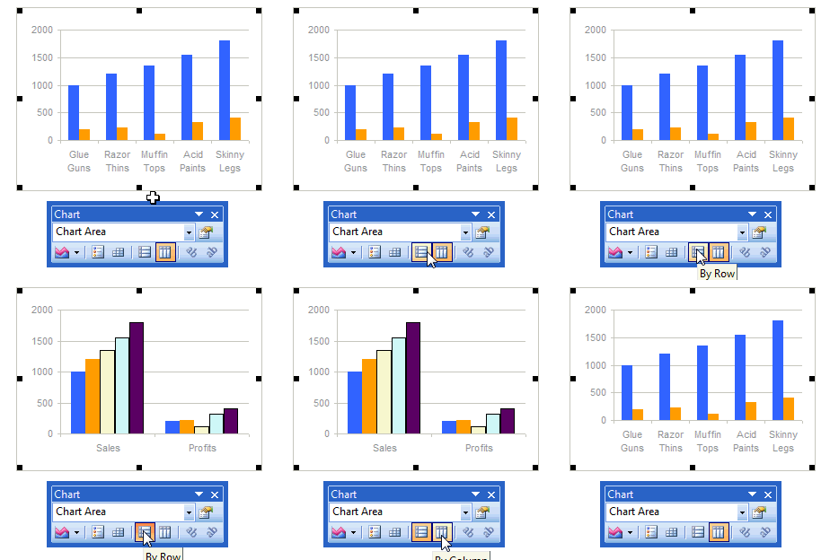
Let us say you have built a nice chart showing your sales and profits for the top 5 products (learn how to highlight top 5 products in a list), with products on X axis. Suddenly your boss wants to switch the rows to columns (or transpose the chart) so that she can see metric level grouping instead of product level grouping. No need to freak out and rush to Espresso machine, You can do it very easily with Excel Charting features.
In today’s quick tip you will learn how to swap chart rows and columns in excel,
In Excel 2007+, select the chart and go to “Design” tab. Here you will see a big-fat-“Switch rows and columns” button. Just click it and thump your chest. See this tutorial to understand.

In Excel 2003, select the chart and in the chart toolbar, you see 2 little buttons, called as “by row” and “by column”. Click the one you want and off you go. See this tutorial to get it.

Read more quick tips and/or charting tips, be awesome at work.


