

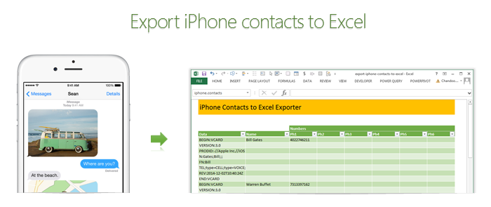
Recently my iPhone 4 crashed. It is 3.5 years old. And just like any other 3 year old, it started acting weird & crazy one night. The next morning it went silent. It won’t go beyond the Apple logo whenever I start it. Since I couldn’t wait for the phone to start, I took out the SIM card (the phone is unlocked, if you are wondering) and placed it in my old Nokia phone. But alas, none of my contacts are on the SIM. They are in “cloud”.
After a day of answering phone calls from everyone including my mom as “Chandoo here”, I’ve decided to get my contacts back. So I logged in to iCloud to download a backup. And the backup was a .VCF file. It has my phone numbers in this format:
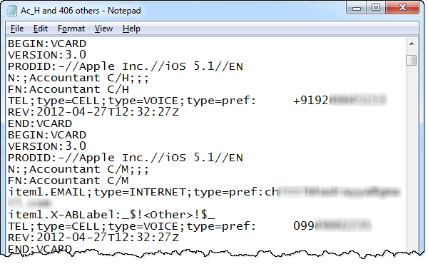
Since I wanted to have all my contact numbers in a spreadsheet, I did what any Excel nerd would do. I built a template for that.
Template for exporting iPhone contacts to Excel
As a first step, download the template.
This template can,
- Export iPhone contacts to Excel
- Create iPhone import format from a list of names & phone numbers in Excel
Exporting contacts from iPhone to Excel
To export the contacts from your iPhone to Excel, follow below steps
- First back up all the contacts on your phone to iCloud
- Now, visit iCloud and select all of your contacts.
- Using the settings gear icon at the bottom, export your contacts to a .VCF file.
- Open the vcf file in notepad & copy everything.
- Paste the data in Data column of “export” tab of the download file.
- Names & phone numbers will be extracted in column D:J
- Filter the table so no blanks are shown in Name column
- Copy the values from Name & phone number columns and paste in a separate sheet or file
- Save.
Importing spreadsheet contacts to iPhone
To copy all your spreadsheet contacts to iPhone,
- Go to “Import” tab of the download file.
- Type or paste your contact information in the columns B,C & D.
- Select “VCF to copy” range (from H4 to last cell)
- Copy
- Open notepad and paste.
- Save the notepad file as contacts.vcf
- Import the VCF file to your iCloud
- Done
Confused about the process? See this video
Since the process of exporting or importing contacts thru iCloud can be a little confusing, I made a small video explaining how the template works. See it below:
(click here to see the video on our YouTube channel)
How does the template work?
The vCard format files are simple text files. So when pasted in Excel, all we need to do is figure out where the contact name & phone numbers are and extract them using, what else… Excel formulas.
Exporting VCF to Excel:
- This uses MATCH formula to find the line in VCF data that has the information we want.
- Then OFFSET formula to extract the corresponding line of VCF data
- And then SUBSTITUTE, MID, LEFT & TRIM formulas to extract the text portions
You can examine all these formulas by unhiding columns C & K:Q in the export tab of the template.
Importing Excel data to VCF:
- This uses INDEX formula to get a name & phone number from entered data.
- Then uses CHOOSE & SUBSTITUTE formulas to create the corresponding VCF lines
- Finally TODAY & NOW formulas to create the timestamp element of the VCF
You can examine these formulas in columns F,G & H in the import tab.
Do you like this template?
It was fun building something useful & immediate like this in Excel. Although, soon after I created the template, my iPhone magically sprung back to life, I will be ready next time I need to look at my contacts or load them to another phone.
How do you like this template? Would you use this or some other app to export / import your contacts? Please share your thoughts and tips using comments.


26 Responses
Any operations on text is to find the pattern which is the tricky part of the problem and next is apply Excel function which is easier part.
Most of the encoded messages in any system will definitely follow a pattern. I have always used this technique to solve my problems with Excel without downloading the small app developed by others for doing the same.
My story of finding the last word in a sentence is at vppc.wordpress.com
Though I hate to publicize but do not have patience to type all 😀
Is this possible with Android devices?
It should be. The VCF format is universal. If you can somehow extract the contacts from Google or other platforms on which they are saved by your Andriod device, you can follow the same steps.
You can export your Android phone contacts from the Google contacts website assuming you have not disabled Google sync on your phone. You get a three choices for the file format – Google CSV, Outlook CSV, and VCF. Choose the Outlook CSV format and open with Excel. It’s very easy. If you don’t use a Google account on your Android phone, then this won’t help.
Since Android does not work, I just did the test, perhaps VCF formats are different.
PS: Sorry for mi bad english!
Thank you for this! It’s awesome!
I just tried this. I followed the instructions perfectly (I think).
I downloaded all my contacts from the icloud in vcf format and saved the file.
I opened the file in notepad and copied and pasted the data into the data in Data column of “export” tab data column (8110 lines of data)
Nothing got extracted into Columns D-J
Now that being said, when I downloaded the template; I got the following error on opening: The file you are trying to open is in a different format than specified by the file extension. (The file extension is xls). I change the extension to .xlsx and the file opens without an error. But still does not do the extract. 🙁
Hi Chris,
Can you first record of your VCF file in comments so that I can examine what is going on. Please post everything between first BEGIN:VCARD and END:VCARD lines. Please replace names & numbers with random data to ensure privacy.
I am facing the same issue. Here is the first entry:
BEGIN:VCARD
VERSION:3.0
PRODID:-//Apple Inc.//iOS 7.1.1//EN
N:;A;;;
FN:A
TEL;type=CELL;type=VOICE;type=pref:123
REV:2014-06-14T09:29:51Z
END:VCARD
I think Mr Modi should have made the big names in your template!
thanks for this post – I also have an iphone 4 on borrowed time.
I downloaded the template, followed the instructions and bingo.
Thank you so much Chandoo.
BLESS YOU CHANDOO! I upgraded my iPhone to a 5S and gave my old 4 to my daughter. I went to switch the account on the old 4 to her account, but I had forgotten her Apple ID password so I figured “I’ll fix that later.” Several weeks passed and little did I know, she was deleting the contacts on the phone because she didn’t need them. Until she came to me and said “you know too many people” I had no idea that she was not only deleting them on her phone, but they were disappearing from my new 5S (thank you iCloud sync) since both phones were connecting to the same iCloud account. After spending $65 on a product to extract contacts from an old backup, I still had no idea how to get the contacts onto my new phone. The extracted contacts are in individual text files. Looks like I’ll be writing a macro to import them into your template and then I’ll be ready for import to my new phone. Thanks again for this!! I can’t wait to try it out this weekend.
Howdy,
Worked pretty well but most of the numbers are missing. Thoughts?
Hi
Slightly tangental question, but wondered if you had come across this –
I have all my contacts in Excel (extracted from outlook and tidied) and then imported into google contacts
the problem i have is in the formatting of some (not all numbers) particularly international ones.
eg + 31 61234567 loses the “+” in excel and then comes out as 3.16E+11 when up loaded to google
is there a way of formatting the international numbers so that the prefix (eg +31) is retained ??
many thanks!
@David.. You can set up the column where these numbers go as TEXT and then import the data.
Hello Chandoo,
I used this template and it worked like you said, but it duplicated the last name twice. It appears that your template is only capturing the phone numbers (which is obviously what you wrote it for), is it possible to expand this template to capture mailing addresses? My goal here is that I would like to create a lookup table in excel to do a mail merge for envelope printing. I keep all of my contacts in my mac.
Thanks so much. You are a lifesaver. I have been trying to figure this out for 2 weeks and found no help from APPLE. They even suggested that I check elsewhere! I will come to you from now on for great – easy ways that even I can get things done without unwarranted spending.
Thanks again,
Sunny
Could this work with Mac’s “numbers” program? Is there a “numbers”
version of this?
Shawn
Hi Chandoo
I got some #values coz my vcard export looks like this (Iphone 4s). I had to hack to get it to work.
BEGIN:VCARD
VERSION:3.0
PRODID:-//Apple Inc.//iOS 6.0.1//EN
N:;Test;;;
FN:Test
TEL;type=CELL;type=VOICE;type=pref:+1XXXXXXXXXX
TEL;type=WORK;type=VOICE:+1XXXXXXXXXXX
REV:2012-12-17T21:01:31Z
END:VCARD
BEGIN:VCARD
The second comment is that ur template takes in only one number but a lot of my contacts have a second or third phone… Any suggestions for that?
What did you change it to, because I am also having the same problem..
Hey Chandoo,
Is the file still linked? I can’t seem to download the excel itself. Thanks for your help mate.
cheers.
Hi Chandoo
This template would be a Godsend if I can get it to work…
When I paste into the column, it says “Data on the Clipboard is not the same size as the selected area, do you still want to proceed?” I select yes, and then after it pastes, everything is in the first column and no phone numbers or any other data show up.
If you can offer any assistance I would be extremely grateful.
Just a side note: The same thing happens when I paste it the right way (meaning that now when I do it, Excel does not give me that message and everything seemingly goes smoothly with the paste-in but still no data in any of the other columns)
Hi Can the app be extended to take more that 100 contacts, say a 1000
@Keith
Yes
Add the contacts
Copy a formula in Column H Down
Remember each VCard has 8 rows, so ensure you end on a END:VCARD Line
Greetings!
While potential or returning clients are browsing on your website, it’s essential for their experience to be a comfortable and easy task while at the same time aesthetically pleasing. How would you like your website to be more attractive and engaging to more clients with the help of web design? If your site is beautiful, can be easily navigated, and the info they need is right where it should be, you can be confident that they will be buying your products/services. All that can be achieved at an affordable cost.
I’ll provide you with a free consultation to show you my web design ideas that best fit your business. I can also send you my portfolio of websites I’ve done in the past so you’ll be more familiar with the work I do. Please inform me about when’s the best time to give you a call. Talk to you soon!
Thank you.
Donna Lee