
This is part 5 of 6 on Profit & Loss Reporting using Excel series, written by Yogesh

Data sheet structure for Preparing P&L using Pivot Tables
Preparing Pivot Table P&L using Data sheet
Adding Calculated Fields to Pivot Table P&L
Exploring Pivot Table P&L Reports
Quarterly and Half yearly Profit Loss Reports in Excel
Budget V/s Actual Profit Loss Report using Pivot Tables
This is continuation of our earlier post Exploring Profit Loss Pivot Reports.
We have learned how to change our P&L report on various data elements. We have seen how the P&L report can be changed with just few clicks.
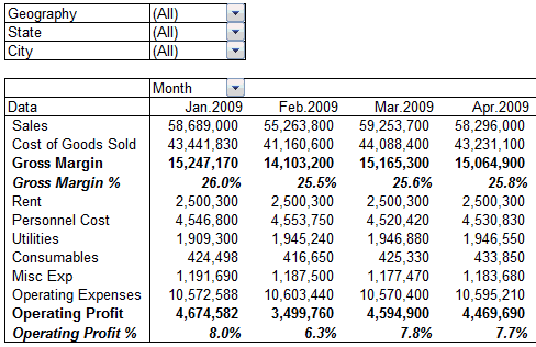
In this post we will be learning some grouping tricks in PivotTables. We will cover grouping of dates, text fields and numeric fields. You will need to start with Monthly P&L report prepared in previous post.
Grouping Profit Loss Report based on Dates
- Right click on date field > Choose Group > Choose Quarters from dates grouping dialog box > click OK.
- Tutorial: Grouping Dates in Pivot Tables.
Once done your quarterly P&L is ready, you can still filter it on any other filed. Checkout screen cast for quarterly P&L prepared and filtered on City filed to make Quarterly P&L for Amritsar City.
Not only this, you can also drag grouped data to page area and Geography field to column area of PivotTable. Now you can filter it on Qtr1 to make Geography wise P&L for Qtr1.
[Click here to see how to do this]
This one is simple as it groups January to March period as Qtr1, April to June as Qtr2 and so on.
Grouping Dates based on Apr-Mar Financial Year
Most of the Indian companies follow April to March as Financial Year. They start with April to June as Qtr1 and finish with January to March as Qtr4. You will need different steps if you want make April to June as Qtr1 and January -March as Qtr4.
In our Data we have January 2009 to March 2009 period as Qtr 4 of 08-09 Financial Year. Grouping steps are as under
- Select January to March month columns > right click on selected columns > Choose Group.
- Rename Group1 as Q4.08-09
- Follow similar steps to Group April 2009 to June 2009 as Q1.09-10 and so on.
- [Click here to see how to do this]
- Drag the grouped field out of PivotTable in case you want to remove grouping.
The final report looks like this:

Many companies follow different Financial Year. In case your company follows May to April as Financial Year, you can select May June and July months and group them as Qtr1. You have the flexibility to select particular periods and group them. You can input name of the group as you want.
In similar way you can group 6 months to make half yearly Profit Loss Report in Excel.
Grouping Profit Loss Report Based on Text Fields
You can group data on text fields. In Geography wise P&L you can group South and East column to make P&L for South East.
You can select non consecutive columns :- Click on East column > Press Ctrl > Click on South column while you keep Ctrl key pressed. You will see that you have both the columns selected.
Select East and South Column > Right Click > Choose Group > Rename Group1 as South East.
Drag the grouped field out of PivotTable in case you want to remove grouping.
[Click here to see how this is done]
Grouping Profit Loss Report based on Numbers
You can also group data on numeric fields. We will make a PivotTable P&L grouping stores based on their size. Prepare P&L on store sizes by dropping store area field into column area of PivotTable.
Right Click on Store Area filed > Choose Group > Enter grouping parameters in Group dialog box > Click OK
You have the P&L for stores grouped based on their size.

Putting it all together – Creating a Custom Profit Loss Report Layout in Excel:
You can explore your PivotTable P&L in any combinations discussed in this post and our previous post.
So how about making South East Geography P&L for Q1 only of stores sized 4000 – 4999, like this?

It is just few clicks and your P&L will be ready , watch out screencast.
[this is a heavy screencast, so click thru if you want to watch it].
Dealing with “Cannot group that selection” error:
While grouping fields in PivotTable you may get a message saying “Cannot group that selection”. This happens due to blank date / number field or text in date / number field. You may have some blank rows in the data causing this problem. Some time you may have second copy of date field shown as Month2 or date2. This is duplicate field created in PivotTable which is already grouped. You will need to un-group this before grouping date filed again differently if required.
Download Excel file with all these example Pivot Reports:
Download Profit Loss Report Excel file and practice all these tricks on your own. [mirror download location]
What Next?
In the next part of this series, learn how to prepare budget vs. actual profit-loss reports.
Meanwhile, make sure you have read the first 4 parts of this series – Data sheet structure, Preparing P&L Pivot Table, Adding Calculated Fields and Exploring Profit Loss Report Pivot
Also check out the Excel Pivot Tables – Tutorial, Pivot Table Tricks, Grouping Dates in Pivot Reports articles to get more ideas.
Added by PHD:
- Say thanks if you like the idea and want to learn more.
- Please share your feedback and ideas for this series using comments. Yogesh and I will reply to your questions.
- Sign-up for PHD E-mail newsletter because you will get updates as new posts go online.
 Yogesh is an accountant with 13 years of experience in India and abroad. His specialties are budgeting and costing, supplier accounting, negotiation of contracts, cost benefit analysis, MIS reporting, employees accounting. He writes about excel at http://www.yogeshguptaonline.com/


