How to present changes in Market Share using Charts?

Share

Facebook
Twitter
LinkedIn

Most of us are comfortable with numbers, but we are confused when it comes to convert the numbers to charts. We struggle finding the right size, color and type of charts for our numbers. The challenge is two fold, we want to make the charts look good (we mean, really… really good) but at the same time we want our audience to focus on the message and not on the bells and whistles. This is where it gets tricky.

Almost 2 months ago our reader Jennifer sent me an email asking if there is an effective way to present market share changes between two periods for 2 products among five competitors.  I have replied her promptly with whatever I could think of as better ways to present the data. But I also posted a visualization challenge: How to show market share changes?

We have got quite a few comments and recently Jon Peltier himself wrote on this here: Show Market Share Changes – Few Alternatives

I thought it would be great to summarize various approaches we discussed as a case-study in how you can take same data and present it in different ways.

This is the data Jennifer had:

Market Share Data - Excel Charting Problem

  1. Here is how she presented it initially:
    market-share-product-2
  2. After seeing user discussions she remade the charts like this.
    Stacked Bar chart and lines showing market share
  3. Derek from Information Ocean responded to the challenge with this step graph (which he admits is not so effective). Nevertheless, they are another fun alternativeStep chart - market share
  4. Derek also proposed this “who is responsible for that?” chart. Despite looking little cluttered I liked this one.
    Line chart - Who is responsible for that?
  5. Dave from Favillae responds with this aligned bar chart alternative to present the same data. Another innovative way, he used blank series to adjust the gaps
    Aligned Bar Charts
  6. Nixnut, a commenter, tried bar charts to come up this variation. These are pretty good and provide both absolute and changes in market share values. He used overlapped chart technique to achieve this.
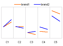
    Bar Charts
    (image url)
  7. Finally the alternatives presented by Peltier.
    This one is a panel chart
    (here is an excel tutorial for panel charts)
    Panel Chart
  8. A stacked bar chart
    Stacked Bar Chart
  9. A line chart
    Another Line chart
  10. A simpler, neater bar chart
    Simple Bar Chart
  11. A panel chart, but this time two products are separated
    Panel Chart with 2 Panels
  12. Last but not least, these are the alternatives I could think of. First one is a Line chart.
    Another Line chart
  13. This is a tag cloud (excel tag cloud tutorial & templates). The fonts are sized based on their relative market share percentages.
    Tag Cloud
  14. And in-cell chart variation.In-cell Chart

Conclusions – Which chart is better?

Well, there were quite a few very good charts. Personally I liked the panel chart version (#7) and bar chart variation by NixNut (#6).

Which one did you like?

Knowing that there are various ways to present the same data and using the version most suitable for your needs and situation is very important. If you want to raise alarm about market share loss, use a chart that alarms people. If you want to downplay the marketshare loss, use a chart that barely shows the information.

Facebook
Twitter
LinkedIn

Share this tip with your colleagues

Excel and Power BI tips - Chandoo.org Newsletter

Get FREE Excel + Power BI Tips

Simple, fun and useful emails, once per week.

Learn & be awesome.

Welcome to Chandoo.org

Thank you so much for visiting. My aim is to make you awesome in Excel & Power BI. I do this by sharing videos, tips, examples and downloads on this website. There are more than 1,000 pages with all things Excel, Power BI, Dashboards & VBA here. Go ahead and spend few minutes to be AWESOME.

Read my storyFREE Excel tips book

Overall I learned a lot and I thought you did a great job of explaining how to do things. This will definitely elevate my reporting in the future.
Rebekah S
Reporting Analyst
Excel formula list - 100+ examples and howto guide for you

From simple to complex, there is a formula for every occasion. Check out the list now.

Calendars, invoices, trackers and much more. All free, fun and fantastic.

Advanced Pivot Table tricks

Power Query, Data model, DAX, Filters, Slicers, Conditional formats and beautiful charts. It's all here.

Still on fence about Power BI? In this getting started guide, learn what is Power BI, how to get it and how to create your first report from scratch.

32 Responses to “More than 3 Conditional Formats in Excel”

  1. m&a in recessionary market says:

    Dude,

    Long time... whts up , I see that urs is the only business which is posting a "Excel" lent growth in this recessionary market....

    Still alive ... so you will be able to reach me if make an attempt... 🙂

  2. James says:

    V E R Y N I C E !!!!

  3. Lincoln says:

    Hi Chandoo.

    When I use your macro in my file, I keep getting a Compile Error because the "cell" variable is not defined.

    Any suggestions?

  4. Chandoo says:

    @Lincoln: Did you have "option explicit" on?

    I am sorry, I didn't define the cell variable.

    you can add this line to the code just below the line "dim i"
    dim cell

    Let me know if you still get this error...

  5. Lincoln says:

    Ah. I've simply declared cell as a range.
    All good now

    Noob at work.

    Thanks for the article. Very helpful. 🙂

  6. Paul says:

    very, very helpful. I didn't know what "define named ranges" meant. one of my colleagues figured it out. I suggest you add the instruction "go to menu - insert/name/define and then make sure the cells at the bottom of the box change to reflect new values if you redefine the range." thanks.

  7. Jahabar says:

    Quite Intresting. If anyone could help. I am trying to do something like this but i want to define values and colours of the value in a range of cells ( Similiar) but i want the other cells to change colour when the value is same as the range defined. ANy help. I want instantaneous( Like conditional formatting) not like running macro.

  8. Chandoo says:

    @Jahabar: Welcome to PHD and thanks for the comments.

    If your source range and target range have same dimensions and source range has 4 different formats (conditional formatting limitation, unless you are using excel 2007) you can do this. If you have more than 4 formats then you may have to use VBA (and create an event like worksheet_change and monitor the range).

    Let me know if you come across a simple non-vba solution for this. 🙂

  9. serdarb says:

    very nice post...

  10. Stružák says:

    May I suggest a little modification of the code?

    Adding "Application.ScreenUpdating = False" at the beggining of the macro and "Application.ScreenUpdating = True" at the end speeds up significantly the whole procedure. As well as omitting "Operation:=xlNone, SkipBlanks:=False, Transpose:=False".

    Not a big deal in this example, but when formatting a larger range of cells, the difference is marked. I've tried to format the number 1457 of cells and the formatting was done 11 seconds faster. :-O

  11. [...] you can overcome the conditional formatting limitation using VBA macros (again, if you are new to excel, you may want to wait few weeks before plunging in to [...]

  12. Hi Chandoo

    Thanks for this macro. I have done few changes to this macro to suit my needs. I had removed the defined names data2use and conditions2use to ActiveWindow.RangeSelection.Address

    This way I can select the cells that require conditional formatting and then run the macro.

    Kind Regards,
    Vasanth

  13. asm says:

    Chandoo, I am using 2007. I noticed the conditional formatting options are different - and they have some built in funtictions for stop light displays, and other dashboard type elements. My question is this, I need to display more colors in the stop light than the standard 3. The World Health Org (WHO) has a Pandemic Flu alert level between 0-6, so i wanted to drive a sharepoint dashboard using excel based on 7 distinct levels. Suggestions?

    • Chandoo says:

      @ASM: very good idea. you can use font based symbols instead of excel traffic light icons to achieve this. the character "=" becomes a small circle when you change the font to "webdings". So you just need to insert a bunch of = signs and use conditional formatting to change the font color. If you need to combine numbers with symbols, then you can use 2 columns instead of one and format them accordingly. Let me know if you need some more help with this.

      Also, if possible, share with us your dashboard when it is ready.

  14. [...] Once we calculate values for all team members using the above formula, we can apply conditional formatting to make the heat map. In Excel 2007, this is one step. In earlier versions of excel, you need to specify 3 conditions to make the heatmap look hot enough or use a macro to get over the 3 conditional formats limitation. [...]

  15. Pitichat says:

    Chandoo,

    Why do you use the "conditions2use" since you can change the VBA and replace "conditions2use" with "data2use" and you won't have to create a zone for conditional formating equal to the data zone.

    The Data will be formated according the "formats2use". Just one thing, if you plan to have some "0" on your data zone, they will be formated like the first cell above your "formats2use" (the green cell with "Formats" inside in your exemple".
    That's why you should leave a white empty cell above the first cell of the "formats2use" zone.

    Regards,
    Pitichat

  16. Justin B says:

    Seeing as no one has posted what they actually might use something like this for here's my 2cents;
    I used the same concepts to build a heatmap of a casino gaming floor, with each populated cell representing a gaming machine (Slot Machine), some simple metric bucketing to determine different shades for the cells, user selectable colours, ability to pick a 'machine' (click on a cell) and repaint the 'floor' showing only machines with similar charateristics, select a value range and repaint the 'floor' showing only the 'machines' within the value range. Users could switch between metrics and repaint the the floor.

    It took a while to put together, but once in use was rolled out to four casinos and used for 4 years. It provided a portable (i.e. no custom software), easy to understand way to manage product from individual machine to groups / classes of product and made it very easy to see how products were performing in geographic relation to each other (something that tables & graphs can't easily do)
    Needless to say it "wowed" many people who only saw Excel as a tool for managing numbers and table based reports
    Being excel just about any user could maintain spreadsheet.

  17. Paul Chapple says:

    @ Justin B - Hey Justin, that counds AWESOME! Can I get a copy of the casino tracker, I work within a similar industry and would love to see how you've constructed it.

    Also, from using this heatmap, I think I'm getting confused. To make the map change color, I thought you had to change the DATA2USE cells, but I see it only changes if you change the vales of thew cells within the CONDITIONS2USE cells. Am I thinking this wrong?????

    Thanks all, this is REALLY making my life easier!!

  18. Rajeev says:

    Hi Dude,

    Thanks for this very useful macro. That was very helpful.

    Kepp up the good work.

    Cheers.

  19. Wagner says:

    Explanation like yours is so important to everyone that want to learn more and more in Excel. Thanks a lot. You are the man ! 🙂

  20. Lee says:

    Chandoo,

    If I wanted to replace the numbers 1-9 with text A-I, what would I need to do to the macro to make it work correctly?

    Thanks!

    • Hui... says:

      @Lee
      If the numbers are alone and not part of larger numbers >10 or with text you can simply use this formula
      =CHAR(A1+64)
      Change A1 to your cell
      Copy Down/Across as required
      Then select the new cells and copy/paste as Values over themselves.

  21. Cathy says:

    I'm trying to do a drop down list that will allow me to select a color and when I select that color it will change my cell to that color. i cannot use contion formating because I have 5 colors. Can you help me with this?
    thanks

  22. Anurag says:

    This tool was great. Can you please suggest a way to include conditions like if value in a cell lies in a range color some other cell red.

  23. CCC says:

    What do I need to change in the programing if I have a mix of numbers and letters.  Example; 5003, 2B01, W005, 1020.  I think the problem is the CInt code but I'm not sure.

  24. Bob says:

    EXCELlent - was able to use your macro with no problems.  Found that modifying it to use the DATA2USE range achived the same result as using the condition2use range.  If the two ranges were equal, your way allows the data range to have completely different values and still have the same color format at the end. 
     
    My data is a little different
    I have an irregular shaped building with students in it.
    I have a list of students assigned to the rooms with the courses they are on
    and a color code for the courses
    would there be a way of using indirect to translate the student names to color code the rooms to what courses they are on?
     

  25. [...] hi Check below link More than 3 Conditional Formats in Microsoft Excel - How to? | Chandoo.org - Learn Microsoft Excel O... [...]

  26. Graham Hartell says:

    The ability to conditional format a range of cells based on criteria in a different, but matching for size, range of cells is exactly what I've been looking for. Unfortunately the macro falls over at the line conditions (i) = CInt (cell.value). I have specified the 3 rangenames, working in excel 2003 but cannot get it to work. Any ideas. I've checked rangenames several times (0-16 being used) but no luck. Thanks

  27. Sebastian says:

    Hello you also can use this code to force ur worksheet to run with more then on condition.
    in this case the condition = case like in example if u want to format something between of the range 0 to 100 for a color
    Set I = Intersect(Target, Range("B2:B8")) <-- thatch the rage u want to work with just set it up for range of cell u want to use to format

    the second formula will show u Interior color nr index just time it and when u format the cell with a color it will show nr in the cell

    enjoy

    Private Sub Worksheet_Change(ByVal Target As Range)
    Set I = Intersect(Target, Range("B2:B8"))
    If Not I Is Nothing Then
    Select Case Target
    Case 0 To 100: NewColor = 37 ' light blue
    Case 101 To 200: NewColor = 46 ' orange
    Case 201 To 300: NewColor = 12 ' dark yellow
    Case 301 To 400: NewColor = 10 ' green
    Case 401 To 600: NewColor = 3 ' red
    Case 601 To 1000: NewColor = 20 ' lighter blue
    End Select
    Target.Interior.ColorIndex = NewColor
    End If
    End Sub

    Private Sub Worksheet_SelectionChange(ByVal Target As Range)
    Range("F1:F1") = Range("F1:F1").Interior.ColorIndex
    End Sub

  28. Tom says:

    Hi Chandoo,

    I tried to add the "More than 3 conditional formats for Excel" VBA macro
    to my Excel 2008 for Mac and it didn't work. Would this VBA macro work
    with Excel 2011 for Mac? Does it have to be a certain version: Student,
    Home & Office, or Standard?

    Thanks for your help.
    Tom

Leave a Reply