
This is a guest post by Sohail Anwar.
August 29, 1994. A day that changed my life forever. Football World Cup? Russia and China de-targeting nuclear weapons against each other? Anniversary of the Woodstock festival?
No, much bigger: Two Undertakers show up at WWE Summerslam for an epic battle. Needless to say: MIND() = BLOWN().

And thus begun one boy’s journey into understanding the phenomenon of Multiple Occurrences.
My journey continued, when just a few years later my grandfather handed me down a precious family heirloom: A few columns of meaningless data that I could take away and analyze in Excel. You may laugh but in the 90’s, every boy only wanted two things 1) Lists of pointless data and 2) To be as bad ass as this guy:

Ohhh yeah.
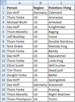
All good but how best to deal with multiple occurrences? Well, it broadly involves a cunning collusion of SMALL, LARGE, IF and our good friend the Array formula. To explain, let’s have a look at one of granddad’s prized pointless lists:
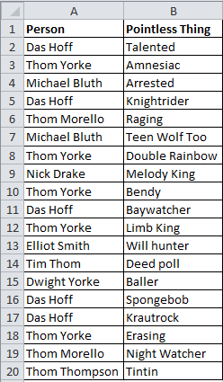
All kinds of repetition of names exist here, so how, for example, can we look up the pointless things about ‘Das Hoff’?

A typical VLOOKUP or INDEX/MATCH combo will give us the first entry (‘Talented’), but what about the rest? The following ARRAY formula will saves us:
SMALL(IF(Lookup Range = Lookup Value, Row(Lookup Range),Row ()-# of rows below start row of Lookup Range)
Entered with Ctrl + Shift + Enter because it’s an Array formula
In this case:
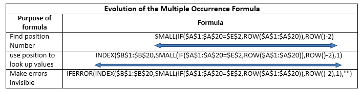
SMALL(IF($A$1:$A$20=$E$2,ROW($A$1:$A$20)),ROW()-2)
Bear in mind this will give us the position numbers of the multiple occurrences in our main list. That’s a good start. Now we drag this formula down so we end up with another list since our need to find multiple occurrences will necessitate creating another shorter subset of the main list, even if there are just two entries. How far do we drag it down? It doesn’t matter too much but enough to capture the likely number of multiple occurrences. we’ll come back to this point in a bit.
I just want to bring your attention to the last part of our SMALL formula, in this case ROW()-2. This creates a rank; think of it as 1st occurrence, 2nd occurrence…as you are dragging the formula down.
Why did I put Row()-2? Well I placed it in a cell which is in the 3rd row and as a rule the first instance of the formula you write, you want the Row()-x to equal 1 (assuming your lookup range starts from row 1). So if your looukup range is in A1:D20 and your first SMALL formula is in cell E5 then you will write ROW()-4 at the end .
Let’s see what happens when we put the formula in E3, search for ‘Michael Bluth’ and drag down to E7:
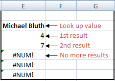
We can visually see there are just two entries in the main list and their position numbers have come through nicely (4 and 7). Beyond that we are met with the #NUM! error. So from here, we need to do two things
- Utilize the position number to give us value or related value from the list (i.e. do what the lookup is supposed to do!)
- Conceal the errors.
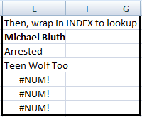
To accomplish (1) we can just put this whole thing into an INDEX formula, define an array size (same vertical dimensions as our main table), use our SMALL formula to provide the row number, then define whatever column number we want, in this case we want column 2:
INDEX($B$1:$B$20,SMALL(IF($A$1:$A$20=$E$2,ROW($A$1:$A$20)),ROW()-2),1)
Which yields:
Now, the final bit involves wrapping all this in our trusted friend IFERROR for some easy tidying up:
IFERROR(INDEX($B$1:$B$20,SMALL(IF($A$1:$A$20=$E$2,ROW($A$1:$A$20)),ROW()-2),1),"")
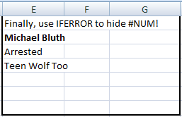
Ta da! Let’s have a quick recap of how we evolved the formula.
What else can we do?
Let’s extend this bad boy formula and make it really work for us. Here are some select ways I have extended the Multiple Occurrence formula to help extract from challenging text data.
Please download the workbook, since it contains the examples for your learning pleasure.
Note: Temporarily for this next section, I am going to ignore the IFERROR and the INDEX parts purely to make the formula slighter shorter and thus a bit easier to read. Instead, what we will get are the position numbers (which are good enough to demonstrate how the formulas work). Relax, in the final section, I’ll bring them back in!
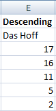
Descending List
Okay, not very exciting, but if we wanted our list to be in a descending order, we simply switch the SMALL with LARGE!
LARGE(IF($A$1:$A$20=$E$2,ROW($A$1:$A$20)),ROW()-2)
Partial Text Search
What if just want to look for part of the text? Easy!
SMALL(IF(IFERROR(SEARCH($G$2,$A$1:$A$20)>0,FALSE),ROW($A$1:$A$20)),ROW()-2)
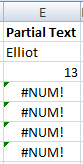
The urge to use a wildcard just won’t work due to the mechanism of an Array. Arrays require like for like comparisons and a partial text won’t correspond to a range. So we need to create TRUE and FALSE outputs, which is what wrapping the SEARCH(…)>0 in an IFERROR does.
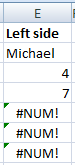
Left side of Text
Let’s say we are looking for a first name in a cell with a full name, we can do:
SMALL(IF(LEFT($A$1:$A$20,LEN($I$2))=$I$2,ROW($A$1:$A$20)),ROW()-2)
Some of you are thinking, well this can be achieved with a partial text search and most of the time you are right. But I routinely deal with tens of thousands of rows of data with varying text and used to fall foul of not preparing for every permutation or combination. It’s subtle but it can be very useful.
Partial text in the right side
‘Now you’re just being silly Sohail! Who needs this?’ I’ll stand by what I said, when you work with lots of data and need to extract all kinds of things, this sort of formula soon finds a place! Unfortunately I can’t reproduce data that I’ve worked with to show you the reality of needing something like this. It’s not often but once in a while it comes and it’s quicker then VBAing!
SMALL(IF(IFERROR(SEARCH($K$2,RIGHT($A$1:$A$20,LEN($A$1:$A$20)-SEARCH(" ",$A$1:$A$20)))>0,FALSE),ROW($A$1:$A$20)),ROW()-2)
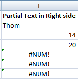
So we’re just searching for things past the first space, this sort of thing would need to be extended as more spaces crop up but you get the point.
Multiple Occurrences and Multiple Criteria!
What?! This is more confusing than making Time Traveling Flux Capacitors.

Okay, to make this work, let’s increase our data set, I’m going to throw in a region column for all the patriots in da house.
So now things are getting interesting. ‘Das Hoff’ is a great example; we can see from a visual inspection he covers two regions (discussing the dual German and US citizenship of the Hoff is out of the scope of this article, but just know how awesome he is!). How can we lookup the two different occurrences of ‘Das Hoff’?
Easy, but first if we harken back to the ultimate VLOOKUP trick I suggested the use of CHOOSE in an array to create ‘virtual’ helper columns, the good news is since we are in an Array format, its pretty straightforward do this without messing with VLOOKUP or CHOOSE. So we simply concatenate the Person and Region ranges and we concatenate the Person and Region lookup cells:
=SMALL(IF($A$1:$A$20&$B$1:$B$20=$E$2&$F$2,ROW($A$1:$A$20)),ROW()-2)
So now if we look up ‘Das Hoff’ in ‘Germany’ and ‘US’ we get:
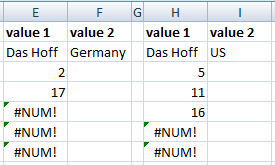
Das ist gut, nein? Ja, Über gut.
Let’s go a step further; what if we wanted to separately lookup the First and Last names? Easy, same concatenation but also concatenate a space in between, like so:
=SMALL(IF($A$1:$A$20=$K$2&" "&$L$2,ROW($A$1:$A$20)),ROW()-2)
So if we are searching for the first name ‘Thom’ and surname ‘Morello’ we get:
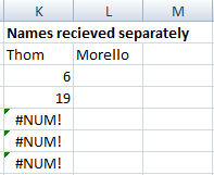
There you have it. Multiple Occurrences WITH Multiple Lookups, take that to the bank!
Autofiltering without an Autofilter!
So, now we have seen the power of what can be done with Multiple Occurrences, how else might we use this in our work? Well, in the Chandoo tradition of creating awesome dashboards let’s build a bit of interactivity in a dashboard. Now I’m not going to build a dashboard, the web’s finest materials on dashboards can already be found on Chandoo.org! No point me recreating. What if we want to create a makeshift Autofilter in the middle of a dashboard/report? We can use everything we’ve learned about Multiple Occurrences and with a bit of conditional formatting we can cook up something pretty decent.

How about we poach the multiple criteria technique from the previous section: First Name, Surname and also Region as drop downs (by using simple data validation lists) to control a table of formulas:
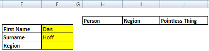
Let’s just look at the formula in each column of the table:
Column 1: Person
IFERROR(INDEX($A$1:$C$20, SMALL(IF($A$1:$A$20&$B$1:$B$20=$F$3&" "&$F$4&$F$5, ROW($A$1:$A$20)),ROW()-2),1),"")
Column 2: Region
IFERROR(INDEX($A$1:$C$20, SMALL(IF($A$1:$A$20&$B$1:$B$20=$F$3&" "&$F$4&$F$5, ROW($A$1:$A$20)),ROW()-2),2),"")
Column 3: Pointless Thing
IFERROR(INDEX($A$1:$C$20, SMALL(IF($A$1:$A$20&$B$1:$B$20=$F$3&" "&$F$4&$F$5, ROW($A$1:$A$20)),ROW()-2),3),"")
The only difference between these is the Column number in the INDEX formulas. Now, I am fully aware of the absurdity of having your search criteria (Name and Region) appear in the results table but it’s cool, I’m just illustrating with minimal pointless made up data. Let’s try using this:
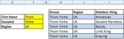
Selecting Thom, Yorke and UK gives us a nice chunky result. And how did we get it looking so slick with expanding/contracting borders and alternating colored rows?! Easy, let’s take a closer look at the conditional formatting:
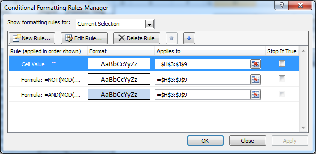
Pay close attention to the order of the conditions, it won’t work properly otherwise. The formulas used are:
For the first condition, I have selected ‘No Color’ for fill:
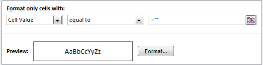
For the second condition, the formula is:
=NOT(MOD(ROW(),2)) – Choose a white fill AND complete Border around the cell.
For the last condition, the formula is:
=AND(MOD(ROW(),2)=1,H3<>"")
The last thing is to turn the grid-lines off or at least paint the cells in and around the table white. Have a look in the workbook if it doesn’t make sense.
Download Example Workbook
Click here to download Multiple Occurrences workbook. It contains all the examples. Play with the formulas to learn more.
Conclusions
So there you go. I hope you have taken away a number of things about the value of extracting multiple occurrences from a list and a technique for enhancing interactive reporting. If there is one thing I really wanted to convey during this article, its how much I love the Hoff and we can never have enough occurrences of this Germanic demigod. If you enjoyed this article then please share it and let’s get a discussion going in the comments to see what other multiple occurrence madness we can come up with!
Added by Chandoo
Thank you so much Sohail for another wonderful, intelligent & useful article. I had loads of fun reading & learning from it.
If you enjoyed this, please say thanks to Sohail in the comments section.
Keen to learn Advanced Formulas?
Check out Formula Forensics & Array Formula pages.
About the author: Sohail Anwar is a Londoner who has spent over 10,000 hours applying Excel in his professional life and earns well over 6 figures as a result. Now he is on a mission to teach professionals how to massively increase their earnings by learning and applying Excel like never before. Find out more about Sohail on Earnwithexcel and connect with him on LinkedIn.


12 Responses to “Sachin Tendulkar ODI Stats – an Excel Info-graphic Poster”
A great tribute to one of the greatest batsmen's in Cricket history.
Thanks Chandoos!
A fantastic poster, Chandoo. I suspect most people would assume it was done in Adobe Illustrator.
Great work!
Daniel Ferry
excelhero.com/blog
[...] Visit his post to download the excel file: Sachin Tendulkar Statistics Excel Infographic Poster [...]
[...] Courtesy: Wikipedia.org >> Chandoo.org [...]
Please update the pingback url to http://www.newsilike.in/sachin-tendulkar-infographics/
Awesome man .....super work
[...] Wikipedia.org >> Chandoo.org ← Previous Next [...]
[...] Kummi in Blog, Dashboard, Excel, Infographic | No Comments Jan252012 Chandoo.org published an infographic poster created in Excel. As a big fan of Tendulkar, I really liked this [...]
[...] Via Tags: europe, football, european league, soccer, sports © 2012 Latest Infographics /* */ [...]
[...] Source [...]
[...] Link [...]
[…] Source […]