
Trust Peltier to come up with solutions for even the most impossible looking charts. Today he shares a marimekko chart tutorial.
 What in the name of unindented VBA code is a Marimekko Chart ?
It is a variable width stacked chart. It is a good way to depict how various segments have performed wrt a set of products, essentially a market segmentation chart. See a sample chart that Jon created to the right.
I couldn’t sit still after seeing his post. So here comes market segmentation charts or marimekko charts using, <drum roll> conditional formatting.
See it for yourself, a market segmentation chart drawn in a 20×20 range of cells.

Here is a brief tutorial on how I created this. With little time and a strong coffee you can build a market segmentation chart too.
1. Adjust the data of your market segments and products
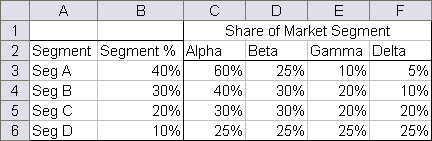
While Jon’s data (image) is oriented such that products are in columns and segments are in rows, I created the below structure as it directly maps to how the chart is drawn (segments in columns and products in rows)

I have derived the below table using formulas. It uses the number 20 (which is the size of one side of our conditional chart) and some rudimentary formulas to derive the numbers 0,8,14,18 from 40%,30%,20%,10% and so on. How ? Now would be the good time to take a sip of that strong coffee and think hard looking out of the window.
2. Create a simple 20X20 grid and start writing formulas
Ok, this is the tricky part. Ideally when the chart is ready we want to have 4 colored regions in each of the 4 segments (this can change if you have more products or more segments). Imagine you were to just write numbers in that grid such that for first product we write number “1” in each segment cells and second product, number “2” so on. Then, color all 1s, 2s, 3s and 4s differently using conditional formatting, then this is how it would look.

Now, we need to just figure out a simple formula that can automatically determine whether to output 1 or 2 or 3 or 4. ENTER THE STRONG COFFEE (or your favorite drink), slurp, slurp…
Ok, did you see those running numbers in the first column and row ? Good, We need to use those numbers to figure out certain things for us.
I have written the following formula in first cell in the 20×20 grid and copy pasted it all over the range.
=CHOOSE(MATCH(I$4,$C$13:$F$13,1), MATCH($H24,$C$14:$C$17,1), MATCH($H24,$D$14:$D$17,1), MATCH($H24,$E$14:$E$17,1), MATCH($H24,$F$14:$F$17,1))
What is it doing ? It is checking which segment the current cell belongs to by matching the top-row number with derived table’s first row (0,8,14,18). So for cell 1 this would be 1, for cell 12 this would be 3. Then, CHOOSE formula uses this information to determine which MATCH formula to run, there are 4 match formulas, each for one segment. All of them check the first-column running number with product-wise start numbers derived in the table 2 above. Slightly lost? Well, me too. Sip once more and read from beginning until it makes some sense.
3. Finally, apply the conditional formatting
Ok, now select the 20×20 grid and apply conditional formatting. Since I have created this in Excel 2007, I could define 4 rules, one for each number. But You can do similar using Excel 2003 (just define 3 rules, one for each number and apply 4th color to the entire range)


Also, hide the cell contents in the 20×20 grid by applying custom format code like this.
Thats all, you are now all set to show off your market segment chart. Go flaunt.
Download the market segment charts template and play around. [Excel 2007 File]


6 Responses to “Make VBA String Comparisons Case In-sensitive [Quick Tip]”
Another way to test if Target.Value equal a string constant without regard to letter casing is to use the StrCmp function...
If StrComp("yes", Target.Value, vbTextCompare) = 0 Then
' Do something
End If
That's a cool way to compare. i just converted my values to strings and used the above code to compare. worked nicely
Thanks!
In case that option just needs to be used for a single comparison, you could use
If InStr(1, "yes", Target.Value, vbTextCompare) Then
'do something
End If
as well.
Nice tip, thanks! I never even thought to think there might be an easier way.
Regarding Chronology of VB in general, the Option Compare pragma appears at the very beginning of VB, way before classes and objects arrive (with VB6 - around 2000).
Today StrComp() and InStr() function offers a more local way to compare, fully object, thus more consistent with object programming (even if VB is still interpreted).
My only question here is : "what if you want to binary compare locally with re-entering functions or concurrency (with events) ?". This will lead to a real nightmare and probably a big nasty mess to debug.
By the way, congrats for you Millions/month visits 🙂
This is nice article.
I used these examples to help my understanding. Even Instr is similar to Find but it can be case sensitive and also case insensitive.
Hope the examples below help.
Public Sub CaseSensitive2()
If InStr(1, "Look in this string", "look", vbBinaryCompare) = 0 Then
MsgBox "woops, no match"
Else
MsgBox "at least one match"
End If
End Sub
Public Sub CaseSensitive()
If InStr("Look in this string", "look") = 0 Then
MsgBox "woops, no match"
Else
MsgBox "at least one match"
End If
End Sub
Public Sub NotCaseSensitive()
'doing alot of case insensitive searching and whatnot, you can put Option Compare Text
If InStr(1, "Look in this string", "look", vbTextCompare) = 0 Then
MsgBox "woops, no match"
Else
MsgBox "at least one match"
End If
End Sub