Today lets close some gaps.
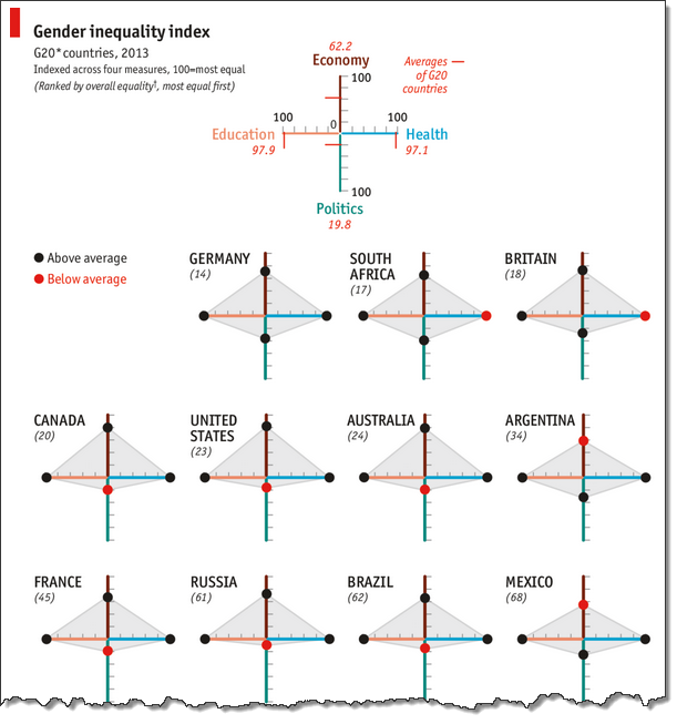
Recently I saw this interesting chart on Economist Daily Charts page. This chart is based on World Economic Forum’s survey on how women compare to men in terms of various development parameters. First take a look at the chart prepared by Economist team.
So what are the gaps in this chart?
This chart fails to communicate because,
- All country charts look same, thus making it difficult to spot any deviations.
- We cannot quickly compare one country with another on any particular indicator.
- It does not provide a better context (for eg. how did these countries perform last year?)
But criticizing someone’s work is not awesome. Fixing it and making an even better chart, that has awesome written all over it. So that is what we are going to do.
Fixing the gaps in Gender Equality chart
First take a look at the improved chart. Play below video.
Step 1: Getting the data for this chart
Although folks at Economist have not included source data, the good people at WEF have provided detailed PDF reports (2013, 2012) where all the data is naked and waiting for us, analyst to pounce and go nuts.
I copy pasted table in to Excel.
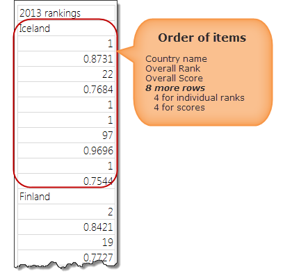
While 2012 data loaded alright, 2013 loaded in a weird fashion.
So we move to step 2.
Step 2: Cleaning the data
I feel dirty every time I clean a piece of data 😉
But I also like it (cleaning part, not feeling dirty part). I learn some techniques when I am working with messy, sticky and disorganized data sets.
The 2013 data is pasted in to Excel in this format.
From this, we need to transform our data to:
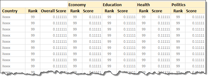
If we know magic, we could point our wand at the table and say something like, Mobiliarbus Datum.
Alas. We are muggles. So lets rely on the most potent magic we know: Excel formulas. Using INDEX + MATCH combination, we can easily convert 2013 data to the format we want.
The actual formula to fetch overall rank (2nd item in the list for each country) is,
=INDEX(gaps2013,MATCH($B5,gaps2013,0)+1)
Explanation:
- gaps2013 is the range where all the 2013 gender gap survey data is copied
- B5 contains the name of the country for which we want the data.
- +1 because we want to get rank, not country name.
For more, read how to get VLOOKUP + 1 item.
Step 3: Set up form controls
Now that we have sparkling clean data, lets create necessary form controls on our output sheet.

![]()
We need 2 controls.
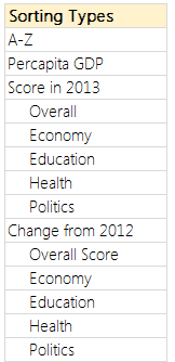
- A combo-box (drop-down) control so that user can select what field to sort the report on.
- A set of option buttons to specify which average to compare.
The combo-box is set up to use the list of values shown aside.
Related: Introduction to Excel Form Controls.
Lets link these to 2 cells, named sortCol & avgType on a different sheet. Call this sheet as calculations. All our formulas will go here.
Step 4: Find sort order based on the selected column
This is the tricky part. I am going to give highlights here and point you to a link where you can learn more.
- Fetch the column we want to sort in a range of cells.
If sorting a number column:
- Make the column unique by adding a very small running fraction.
- This ensures that if our data has duplicates, still our formula works.
- Find the sort order of each item using RANK() formula.
- Refer to Sorting KPIs using Formulas article for more on this technique.
If sorting a text column:
- Find the sort order using COUNTIF() formula.
- Refer to sorting text using formulas article.
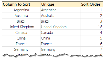
Step 5: Re-arrange all data in the sort order
Using INDEX formula, rearrange all data according to the sort order.
Step 6: Calculate % change values
Based on 2012 & 2013 scores, calculate % change and place them in the last 5 columns.
Step 7: Calculate averages
Calculate averages (both G20 & all country values) for all the columns and place them somewhere on your calculations worksheet.
Related: Calculating the average of every nth item.
Step 8: Create charts
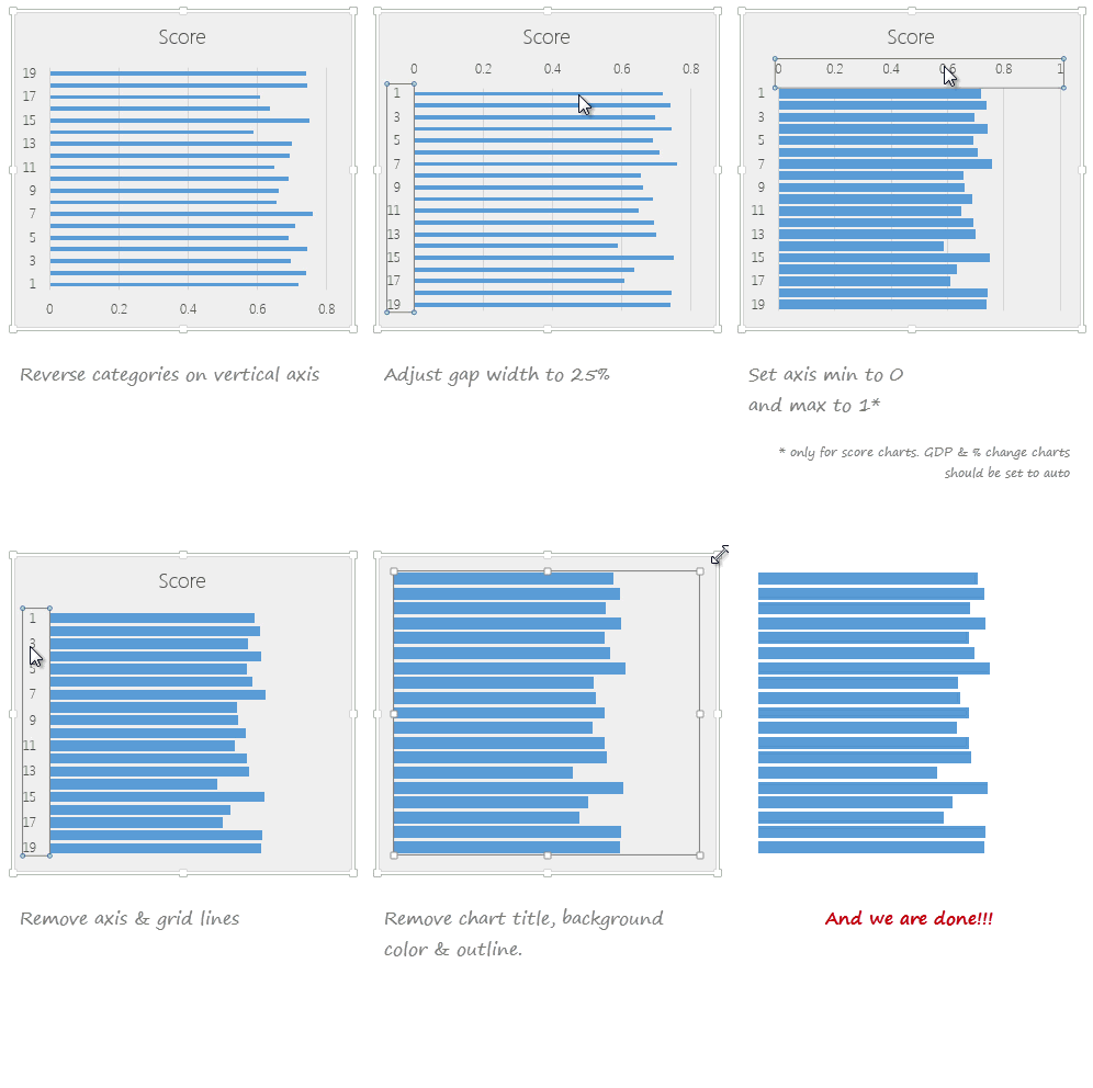
Here is the process for creating chart for Overall Score (2013). The same process is used to create all the charts.
- Select all the numbers in overall score column.
- Create a bar chart
- Select vertical axis and press CTRL+1 to format it.
- Select “Categories in reverse order.”
- Adjust series gap to 25%
- Set horizontal axis min to 0 and max to 1 and remove the axis.
- Remove vertical axis, grid lines
- Remove title
- Fill chart background & plot background with no color.
- Set chart outline to no outline.
- And you are done!
See the demo aside to understand the process.
Step 9: Add average as secondary series to the chart
Calculate which average to use in the chart based on the avgType value. And fetch that number to a cell.
Now add average to the chart as a line. This can be done by,
- Adding average point to the chart as second series
- Converting this series to scatter (XY) plot.
- Adjusting the X & Y values of the average point.
- Adding 100% positive (or negative) error bar
- Formatting the error bar to make it look like a line.
- Removing any axis, grid lines added in the process.
Step 10: Oh wow, this is getting long. Have a coffee
I guess this is now a fairly long process. But closing gender gaps (or gaps in the gender gap chart) is never easy. So have a cup of coffee or tea. Rejuvenate and come back.
Step 11: Create all other charts
Follow the same process and create rest of the charts.
One easy way to create rest of the charts is,
- Copy the first chart and paste it elsewhere.
- Select the bars and edit the range address in the formula bar.
- Select the average point and edit that too.
- Adjust axis if needed.
- And you are done!
Step 12: Put everything together
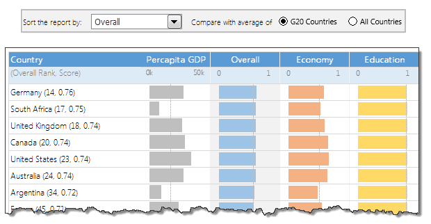
Create a nice table like structure in your output tab and put everything together. Re-size and position the charts as needed. Make sure the colors are nice. Add conditional formatting to highlight column being sorted and you are done!
Missing Steps
I have deliberately omitted a few steps in this process to keep it simple. For those of you with a keen eye:
- Using conditional formatting data bars for the % change column.
- Turning on / off last column in the report based on sort selection using conditional formatting.
- Adding data labels to the country names based on the sort selection.
Download this Excel chart
Click here to download this Excel chart. Play with it. Explore the chart settings, formats, formulas and controls to understand it better.
Conclusions – What does the Gender Inequality Chart say?
After all this analysis, 2 things are clear.
- In most countries, women have high equality with men when it comes to health or education.
- The real gap seems to be in politics & economical development of women.
While this may seem like common sense, it also means, World Economic Forum people should measure inequality on some more parameters. There is little point tracking and analyzing indicators related to health or education (especially in OECD or Western countries).
What do you think?
Want to fill gaps in your Excel knowledge
While no one appreciates gender inequality, we all love awesomeness inequality. There is nothing wrong in wanting to be more awesome than your peers. And here is how you can be unmatched…
- Using Panel charts to understand data
- Spot matrix charts – alternative to radars
- Analyzing performance of stocks using charts
- Suicides & Murders data – interactive analysis
- Visualizing world education rankings
- Survey data analysis with in-cell charts
Want some challenge… How would you analyze this data?
If you want some challenge, go ahead and download the file. It has all the data for 2012 & 2013. Analyze it and share with me your charts. You can email me at chandoo.d@gmail.com or upload your files somewhere and post the links in comments. I would love to see how you can analyze and present this data.


132 Responses to “Excel Tables Tutorial & 13 Tips for making you a Data Guru”
Chandoo, I have only been using data tables for a few weeks & have discovered that they can be used to have charts dynamically expand to take in new data.
Simply set up the chart data in a block with appropriate headings (headings must be text, not formula).
Convert it into a table, select the whole table and insert a chart.
Format the chart as required.
When new data is added the the table and chart will expand to show the data.
The only problem I have found is that the last column of data must show a number when inserting the chart- a blank, #N/A and perhaps text will cause wierd changes in the chart. However this only occurs when first inserting the chart once set up it accomodtes blanks & #N/A etc. This is easily over by adding a temporary number when required on setting up the chart then replacing it with the correct formula when the chart is complete.
This seems to be a lot easier than using offset formula for the series .
Nice post. I've been using Pivot Tables for years but haven't used the "table" button until now.
This is great! Never used data tables before but it helps a lot. One question though, if I try drag your SUMIF formula across a row, different columns are selected in the formula. Normally you can make the columns static in a formula by using "$" - any suggestions on doing the same here?
Convert the data to range. Enter your SUMIF formula, then convert it back to a table.
This doesn't work....well, it only worked one way when I tried it. I had the data as a table and had created some SUMIFS formulae on another sheet. I coverted the data table to range and the formulae all changed to use range references. But when I changed the data back to table, the formulae stayed the same.
Creating absolute structured references is a bit awkward but not difficult.
Some Column as a relative reference
=SUM(Table1[Some Column])
Some Column as an absolute reference -- repeat the column name
=SUM(Table1[[Some Column]:[Some Column]])
The Some Column cell of the current row as absolute -- repeat the column name -- with the Other Column cell of that same row as relative
=SUM(Table1[@[Some Column]:[Some Column]],[@Other Column])
The range of Some Column to Other Column as entirely relative -- repeat the table name
=SUM(Table1[Some Column]:Table1[Other Column])
Nice post. Nice to see such useful options in 2007.
hi Chandoo,
How do you "record" the screen captures of the screens that you need to show into the animated gifs? Do you use a special software for it?
Use the snipping tool on the start menu.
You're posting 4 years late... and I'm posting 5 years late.... 🙂
I use Camtasia to record and produce these animated gifs. You can get a trial version here: techsmith.com
Thank you. This is truly a gem that will save hours and hours of time.
Nice post! However, in a basic form this functionality already existed in Excel 2003 as a 'List' (ctrl-L). So it not needed to convert the table back to a normal range for excel 2003 users.
Chandoo,
nice post. Seems to be a useful feature. Does data tables exist in Excel2003 as well?
@Peter H: Very cool tip about the charts and data tables.
@Dan: Tables are very useful and simple. Pivot can be very powerful for data analysis, but tables are good for maintaining databases.
@Michelle: The sumif formula in the article is written outside the table in a cell. If you write formulas in and copy (ctrl+c) and paste them, then the references are not changed. But if you drag the cell (thus auto-fill), then the cell references to table columns are changing. Not sure why excel would behave like this.
Also, inside the table, you can use [#this row] operator to calculate values for that row alone.
@Frederick: I use camtasia studio to record the screen. It is a nice software. You can test it from techsmith website.
@Doug: You are welcome 🙂
@Robert: My mistake, I meant version earlier than excel 2003.
@Michael: yeah, they are called as Lists. Press, Ctrl+L to create one.
[...] since I have learned the tables feature in Excel 2007, I have fallen in love with that. They are so awesome and so user [...]
i kept saying OMG WOW THATS AMAZING over and over.
i'm quite new with excel so your blog helps a lot and this post, is truly great. thank you!
[...] Microsoft Excel Table Tips and Tricks – Learn Data Tables and Become a Data God | Pointy Haire...By chandoo.org October 16, 2009- ???????Excel???????????????……?X?…… [...]
[...] Microsoft Excel Table Tips and Tricks – Learn Data Tables and Become a Data God | Pointy Haire...By chandoo.org October 16, 2009- ???????Excel???????????????……?X?…… [...]
[...] Microsoft Excel Table Tips and Tricks – Learn Data Tables and Become a Data God | Pointy Haire...By chandoo.org October 16, 2009 [...]
4. Bye, bye cell references, welcome structured references
it does not beat absolute reference to cell i.e $A$1, because if named range is used, it will not copy correctly if u use cell dragging horizontally... it will move to the next name range
This is a huge negative for "structured" references. Excel created a nifty tool that requires me to accept a significant loss of functionality if I decide to use it. It also prohibits dragging cell references to change formulae, so if I drag to fill, I have to click into the cell to manually edit the reference cells to what they should be instead of being able to drag the cell reference box back to the correct column. A small step forward and a giant step back. Or, more succinctly, Microsoft - 'nuf said.
Thanks for the information. Disappointing answer but helps solve my problem.
Chandoo,
I have a question on this. In my sheet I have the "Total Row" added. In that I take an average of a column values and I need to reference this final Average value elsewhere. How Can I reference this specific "totalled average cell" such that when new rows are added the same cell is taken?
As of now, since the total is at the bottom of the table, when a new row is added the cell id of this "total average" row keeps changing. I tried to move it to the top of the table to keep it constant but I couldn't.
thank you
sb
@SB.. you can use the [#totals] tag in the structured reference to total row else where like this:
=Table1[[#Totals],[Column1]] This will work even when you add more rows to the table.
Hi Chandoo,
when i use this code it always shows a #Ref! error.Can you please help me to fix it?
Thanks!
Siddhant
Thanks @chandoo.
[...] will save precious amount of time when you are busy modeling. (100s of tips on keyboard shortcuts, excel tables, formulas, charting & [...]
[...] Select your list of products (or invoices or cats) and make it in to a table. (here is a helpful tutorial on excel tables). [...]
[...] Simplifying data analysis with Excel Tables [...]
Dear Chandoo (Excel Guru)
Thank you very much for sharing such useful tips... now I feel more confident in analyzing a data with Excel....
Regards
Chandoo,
Where referecing table columns as range input to formulas such as sumif(), is it possible to get Excel to treat the reference as static for "fill" purposes?
Cheers,
Steve
@DangerMouse.. you can use ctrl+c ctrl+v instead of drag fill technique to treat the table references as static.
How to make absolute reference on Table column?
I have Table1 and use such formula:
=SUMIFS(Table1[Pay],Table1[Month],G9)
I want to “freeze” columns “Table1[Pay]” and “Table1[Pay]” in formula (like $A:$A).
How to do it?
Looking at article like these make me sad 🙁 - still being laden with 2003 really goads when you see so many fantastic improvements just out of ones rech like this......
[...] Excel Tables, a newly introduced feature in Excel 2007 is a very powerful way to manage & work with tabular data. I really like tables feature and use it quite often. If you are new to tables, read up Introduction to Excel Tables. [...]
I want to learn some excel course from you.
If you have any training centre in Mumbai, Please let me know..
Excellent Work!
Thanks
Avinash Ahire
i want to learn some advance tally course from you
if you have a training center in mumbai any location, please let me know
Excellent work!
[...] 10 Tips on using Excel Tables [...]
Is there a better way than ctrl-c-ctrl-v to expand the ~ifs() formulae across a row while keeping the absolute references to the auto-named ranges in the data-table? I know this has been mentioned a few times in the comments but I'm hoping someone cleverer than me might re-look at this...
All I've got so far is transposing my new table I'm trying to create so I'm dragging down instead of across, which holds the named column references, but I would prefer a dragging across solution
This is my first post on your website Chandoo, but I've been reading for a couple of weeks. It's a fantastic site! Thanks for all your efforts
I love it, I love it, I love it. Don't know how many errors I run into because of bad cell references this should help mitigate this.
Ok REALLY stupid question, I created the table and I have been putting in formulas using the column names, how do I "without using my mouse" select the table name from the tool tip ( or drop down) that shows up. Currently I have to scroll my mouse down to the right column name and then click it add the bracket etc. This also applies for when I use formulas in general. Please help, I am trying to be "Mouse free" 🙂
I have been using Excel forever this is amazing.
Hi Chandoo,
I am using Excel 2007.
I am using an excel workbook to enter data for several different sites (each site has its own worksheet). I want to establish a summary worksheet showing the consolidated data accross all sites so as I enter data into the individual site worksheets the data is also replicated in the summary worksheet which is then sorted by site to show the consolidated view of all sites. Each of the site worksheets have the same data headings which will be replicated in the summary worksheet.
Can you please give me some advice as to how I can go about this?
I know how to use the basics of excel but know nothing about using databases like Access so I would prefer to continue to gather the information in excel if this can be done.
Hoping you can help me,
Jim Morley
[...] The Data Table function should not be confused with the Insert Table function. [...]
[...] Excel 2007, Microsoft has introduced a powerful and useful feature called as Tables. One of the advantages of Tables is that you can write legible formulas by using structural [...]
Chandoo,
I really missed you discount offer last week or so,That day i could not access the internet.Any chance of getting discount offer, i am really interested in joining your course.pl let me know.
Chandoo, thanks a lot for all your tips and tutorials. Your tutorials are really great and easy to follow!!!
Hi, Can i access Excel 2007 table via code - JavaScript?
WOW!
I've spent days organising a "table" of my own (without knowing it) writing formulas,creating helper columns and generally getting stuck and i just figured out that tables and pivot tables do all this in minutes. I dont know whether to feel downhearted or elated that i've learnt this! (all be it too late)
[...] Learn Conditional Formatting 3. Making Dashboards using Excel 4. Project Management with Excel 5. Working with Excel Tables Topics & Archives 1. Learn Excel - Topic-wise 2. Charting Tips, Tricks and Tutorials 3. Ask an [...]
Hi ,
I need a vba for excel training in delhi, kindly suggest regarding this..
How do I get the AutoFormat of Double-Bars in XL 2010? It was so easy in 2003, but I cannot find a way to do it, w/o VBA, in 2010! It can't be that hard.
In 2003, Format, AutoFormat, choose the List 2 style. It formatted rows in groups of twos, or pairs. Very handy in lots of cases.
Any ideas?
Thanks
[...] Learn more about Excel Tables. [...]
[...] How to Use Tables to Speed up Formatting of your Data [...]
I have become a fan of tables now. 🙂
Hi Chandoo,
I used structured reference but when I close and open again, they have all become cell references! Is there a way to fix this? I am using 2010. Thanks,
Prem
Even I have the same problem and worst is it when we add new rows the formulas now do not get changed as it is now having cell references 🙁
Regads,
Prasad DN
Make sure you're saving in the 2007 or 2010 format (instead of the 93/97 format).
Dear Sir,
i want tech the micro soft excel data table and function for opperating the micro soft excel. please give send the tip of micro soft excel.
with best regards and wishes,
Muhammad Bilal Yousaf
Dear
I went to some new learn work in excel
latest
best Regard
Farooq Asim
Absolute references:
As Chandoo says, these move if you use drop and drag. However, if you highlight the required cells, place the cursor in the cell to be copied and use Ctl Enter then the formula copies keeping the references "absolut"
Linda
Good work done.
[...] have set up this data in an Excel Table called as tblSales so that it is easier to write [...]
I've tried to name tables so that I can reference them in functions, etc... but I'm not having any luck getting the name to stick. I can click in the area to the left of the function button and type a new name for the table, but clicking outside of that causes the name to revert back to what it was (for instance, 386, or 3). Thoughts?
@Eric
Select any cell in the Table you want to rename
You should see a Table Tools, Design Ribbon
Select that Ribbon and on the Left there is a Table Name: dialog
Change the name and press Enter
[...] wrote a great post several years ago that explained the basics of Excel tables and provided a number of tips and tricks related to them. [...]
How to rename a Data Table name in Excel.
Sorry guys i got it.
i like you your website, but i quesestion i wil written to excel in accountant but evry time name party not incuding, so anything i find to party name is all ready this excel in ready name ,so you my question solve and reply to me my email id vimal_jariwala15@yahoo.ca
Nice Article
Hi,
How can one add zebra lines in table rows in Office 2010?
@Nitin K.
When you say Table I assume you have a Table setup using the Insert Table menu
If so goto the Table Tools, Design Tab
Select one of the Zebra styles or edit one to setup your own colors
If you don't have a Data Table, select your Data and goto Insert, table menu, then follow the instructions above
You may also want to have a read of: http://chandoo.org/wp/2011/12/08/formula-forensics-no-005/
I have learned so much in the last few weeks since joining in here. Well done.
Now I have a query that I need hlep with. The company I have started working for uses loads of data. Reports are exported to Excel then sorted etc etc...
The Key ref numbers are numeric, 12345.1 and 12345.10 etc etc. Excel will obviously sort the .10 above the .1 - Its an habbit of the reporting software to create a .1 and not .01 Is there anyway within Excel to block alter all the .1's to .01's? I'm talking thousands of them, not just a handful that could be formated as text manually.
[...] Use Excel Tables: Since Excel 2007, we can create tables from structured data and write formulas, create charts that refer to dynamic ranges with ease. Click here to know more about tables. [...]
[...] the dashboard on the Property Register converted to an Excel Table (a 2007+ feature that many are still unaware of) enables the use of Slicer selectors in Excel 2013 to quickly give a dashboard feel. It’s [...]
Great site, and your instructions are so easy to follow. Thanks so much!
On sheet 1, I have a table of names and demographic information for each.
On sheet 2, I am using the same table of names but different data across the columns.
When I add a New Name to the table on Sheet 1, I have to manually extend the table on Sheet 2, to expose the new name.
Is there a way to automatically expand the table on sheet 2, to show the new name added to the table on Sheet 1??
Thanks so much
Has anyone tried using named tables as data sources outside of Excel? For instance, referencing the table for a mail merge? If so, how have you got it to work? Thank you all!
Yes. I use tables in a mail merge. There's no trick (I can think of) to it different than using any other Excel data to mail merge. My own notes for mail merging mention that I open the Excel spreadsheet first and that I need to make sure that the active sheet is the sheet with the table I want to use on it. I do seem to have had problems if a different sheet is the active one.
There IS a trick to making sure your Excel formatting (like number formatting for $, etc.) comes through. But that is true whether or not you are using a table.
[...] of data in this dashboard is captured using Excel Tables. This has several [...]
I like to say, "If you're not using tables, you're doing it wrong." Or at least 90% of the time you should be using them!
I would like to say, "Tables are the best thing since sliced bread", but it then occurs to me that sliced bread is highly overrated. I can slice my own loaf much quicker than doing many of the things manually in Excel that tables make easier.
I LOVE tables! They have changed how quickly and awesomely I can analyze and present data.
Hi Chandoo, another awsome tutorial.
Can you expand the VBA so that i can leave some categories blank and the table will show ALL entries for that category? (eg all Customer Types or all Regions)?
Thanx, Gijs.
[...] ourSales[month] refers to the month column in the ourSales table. Works only in Excel 2007 or above. Know more about Excel Tables. [...]
So I created a data table and wrote forumlas using the data table and column names. It all calculated out beautifully. HOWEVER, now that I want to add lines to my data table, none of the formulas are seeing the added data. I've gone in to expand the range of the table, etc. But still no luck. So stinkin' frustrated :/ Any advice??
[...] best way to create a tracker is to use Excel tables. Set up one with 4 columns – Employee name, vacation type, start date & end date, like [...]
Hi,
I need to convert some data into columns can anyone help me?
[...] Visit link: Microsoft Excel Table Tips and Tricks – Learn Data Tables and … [...]
Dear Chandoo,
I have done much research and your Excel offering is certainly highly rated and I would like to subscribe. I am using Excel 2011 for Mac. Will the course content be compatible? I assume it will but perhaps you have been made aware of some idiosyncrasies?
I look forward to hear from you.
Louis
P.S. Are you aware that your reference to "GOD" will be offensive to many in the Biblical-based faith community (of which I am a practising one)? I suspect you are using it in a different context but it does detract from your brilliance.
[...] how your data for the projects/entities being tracked laid out. We will use the Excel data tables [structured references] to help us [...]
[...] how your data for the projects/entities being tracked laid out. We will use the Excel data tables [structured references] to help us [...]
[...] created an agenda table with below [...]
[...] Introduction to Tables in Excel [...]
[...] select any cell in range and press CTRL+T. Specify a name for your table from design tab. Read introduction to Excel tables to understand [...]
[...] Introduction to Tables, Introduction to structural [...]
Dear Chandoo,
Just one word "Amazing" I like this site 😉
Thanks for sharing all of these
Good Luck
[...] wrote a great post several years ago that explained the basics of Excel tables and provided a number of tips and tricks related to them. [...]
hi chandoo,
I m unable to get the point 6. plz help.
@Arindam
The Menu's Chandoo shows as Pt 6 vary from Excel version to Version
They are accessible by
Click in a PT anywhere
A menu Bar will appear with Pivot table Tools
It may have a Options Tab and a Design Tab
Select the Design Tab
You should see the options shown in Pt 6 here
[…] am sure you all are aware of a feature called as Excel Tables OR Structured References in Excel. Excel Tables is (in my opinion) the best way to store your raw […]
Hi, in point number 6 of http://chandoo.org/wp/2009/09/10/data-tables/
Total your Tables without writing one formula
The ability to summarize data with pivot tables is extended to excel tables as well. You can add total row to your table with just a click.
What more, you can easily change the summary type from “sum” to say “average”.
How do you change the summary type from sum to say average?
@Mona
These are pivot tables
So simply right click on the Total line and change the Calculation type from Sum to Average
Table Text Filtering - is it possible to have column 1 ( in this case named "WO") in the table filter automatically based on the date referenced in another worksheet cell within the same workbook?
Thank you 🙂
Excellent presentation...it would surely interest the most excel fearing people I knw
[…] LinkExcel data table is a series of rows and columns with related data that is managed independently. … Excel 2007 has some great pre-defined table formatting opt…chandoo.org […]
how can add last paid amount in vacation track.
[…] Tables: to keep the products & services data […]
Tried removing the filters but it was difficult. Any reason for this?
Valuable information. Fortunate me I discovered your website unintentionally,
and I'm surprised why this coincidence did not came about earlier!
I bookmarked it.
Going to drop this comment here, since I could not really find a suitable post otherwise. I am not sure if I am overthinking this per usual and missing a very simple remedy - but nonetheless I find myself at a dead end.
Anyone know if it is possible, and if so, how to have multiple headers in a table? I know it sounds counterintuitive but I would like a way to pivot a bulk set of data (set in an Excel Data Table) but have the option to choose 1 of 2 Options when choosing my data header for the Pivot.
Let me try and explain a scenario. So each row has an Account, Part #, a specific week ending date units sold, and a specific week ending date unit dollars. For each account, we sell maybe 5-7 products. So Retailer A has 5 unique rows, Retailer B has 7 unique rows, yadda yadda.
I have 4 tabs, very similar of one another, the only variable is the year (specified by the tab) - or - table name ... and the removal and inclusion of obsolete and new products.
Our Sales weeks are Sunday-Saturday. So, I have 2 column headers that read 11/15 Units and 11/15 Dollars; for this past week.
However, If I wanted to compare this past week to last year or 2012, using Power Pivots, I would not be able to - since "week endings" do not lineup. That is to say in 2013 Week 46 (this past week-end week) correlates to 11/16.
So I would not be able to do a 1:1 comparison easily within a Pivot due to the variation in dates. So logically, I would need some sort of common denominator. I would imagine this would be Week "X." So essentially two separate (or hierarchy?) column headers. I would either need "Week 46" act as a parent - above both "11/15 Units" and "11/15 Dollars" ... or alternatively two separate "co-headers" right above them: "Week 46 Units" and "Week 46 Dollars"
This way, I could compare multiple Week Ending sales data, across multiple tables, using a Power Pivots, based on a common property.
Does anything like this exist? I feel like I would have come across it by now if it does.
And to note, I cannot simply just change the way we handle data to reflect a Week # and omit the XX/XX date methodology. I wish I could, cause that would be abundantly easier.
@Mark
Can you post the question at the Forums and include a sample file?
http://chandoo.org/forum/
Not sure how 11/15 or 11/12 can reference a week as it refers to a month!
If you use the function WEEKNUM(date) with date being the date of the Saturday or Sunday, it will refer to the same week whatever year you are looking at.
So your "co-headers" could be =WEEKNUM(date)&" Units and =WEEKNUM(date)&" Dollars".
[…] Excel Data Tables – An Excel table consists of a series of rows and columns with related data that can be managed independently. Most work in Excel happens inside a table. A table allows users to easily create formulas to make calculations related to one or more rows and columns. Some examples of formulas include the sum of a column, an average, a maximum or a minimum value. For more on tables, visit this tutorial. […]
very useful informations. billion thanks.
Why using tablet format on a file makes it so big?
I had to change all my formulas to references because the size of my file was to big to work.
Any advice ?
Hello Brother,
Your website is awesome. Thank you for all your work. I cannot be as your ordain in your 3rd paragraph as I believe in the One, True, Almighty God. But I can try to be the best I can.
Thank you sir for all your work and sharing.
Chandoo,
As usual, this article was very well done and I thank you for sharing. I'm posting this comment about some trouble I had with Tables, just as a warning for others who might stumble into it, too.
So readers know how much time this cost me, I'll admit this issue took me down a 5 day journey, including an Office 2010 Repair, then an Office Uninstall both of which threw similar errors, so I found an MS Fixit Tool that seemed to describe my situation and ran that but it, too, threw a similar error, and then found a 3rd party utility that claimed to clean up the residue of Office Uninstalls that went wrong, but, it, too, threw the same similar error, but it did at least remove Office from Programs and Features, so I proceeded to re-install Office but that re-install also erred out with the same similar error. After scouring the Internet for this error as well as the original issue (below) that made me think something was wrong (and unbeknownst to me that the cause was a Table issue), I concluded that I must have a virus on the system (despite being current on all my Updates and running 24/7 Virus and MBAM anti-malware) and proceeded to do a clean re-install of Windows 7, Office 2010 (as well as all associated Windows Updates, all my browser Add-ons and preferences, and all my programs, etc. but I took the time to also do something I should have done a long time ago and set up a cloned image of my hard drive when done so if I have any further issues, a re-install of Windows and everything else will be a 20 minute walk in the park instead of the nightmare this has been.
Anyway, back to the Table issue: While working on a large project that has some 10 Tables in it, one of which had Table Headers that were formula driven (these were incremental Date Formulas), that somehow were subsequently getting Pasted as Values. I was building these Tables with Code, and therefore wasn't seeing the warning that Converting a Range to a Table would convert Formulas to Values (and since I hadn't ever done this before, didn't know that message presented if done manually). In my subsequent endeavors to go back to earlier versions where the formulas were still dynamic, I found I could Copy the formulas from the older files, but no matter what I did, I couldn't Paste them as Formulas. This capability is an essential part of Excel, of course, but it wasn't until I had re-installed Windows, Office (et al), and found out that the problem was STILL there, that I finally figured out that it couldn't have been a virus, and finally moved the file to another PC, where I confirmed that the problem was in THE FILE. So, amongst many lessons I learned in this journey was that if you have to have Formulas in your Table Headers, then build into your code (or manual process) a routine that places a copy of your header row under your 'nominal' Header Row (and hide it so you don't have duplicates), but reference the hidden row as your Table Headers.
Hope this helps someone as there is a LOT of other forum posts out there that have to do with Excel Copy/Paste issues but I did not find this as a cause).
In excel Table a copy paste is not working the way it should. Within a Table I am trying to copy a cell's content into another cell it copies totally different value. Need assistance on how to deal with it. Thanks.
I found that I can not paste values in cells within a Data Table- whether they are copied from within the table or outside it (although the cells in the Data Table have NO foumulas!).
I hope someone has an answer to this (i've been searching for a long time).
Hi Chandoo
I'm trying to get my head around Excel Tables and Structured Referencing
and struggling to see how something like the following could be accomplished using this methodology: IF "A1" AND "B1" ARE BLANK AND "C1" AND "D1" ARE NOT BLANK AND "E:E,E1>1", "DUPLICATE","UNIQUE". is it possible?
When the header positions change my formula take the original header positions' data. How do I address the issue?
pls l need you to teach how to use excel from the beginning l have lost touch about some of the functions
IF I HAVE DATE AND PLACE IN ONE COLUMN HOW CAN I MOVE IT INTI TWO COLUMNS
27/05/1956 OVL-DELHI
10/09/1956 AHMEDABAD
30/01/1961 DELHI
Hi. Thanks for having this amazing web site. I wonder if excel tables have the capability to add more than one total row.
Thanks,
[…] The vertices of the regular octahedron with its centre at origin will be as below. let us enter these in excel worksheet as Dynamic tables […]
Once a table is created how is it updated? Say that the table needs to be updated with changes once a month besides VBA and doing it manually how is data refreshed in a table? Is there an Excel formula or module to make changes?
This is an amazing post. Have been using Excel for about 8 years now but never came across this.
Thanks a ton, Chandoo 🙂
Tables make it easy to create dynamic charts, but how can you use the filtered data to create a dyanamic title - eg checking that there is a unique value in one column and then using that?
[…] Excel Data Tables – An Excel table consists of a series of rows and columns with related data that can be managed independently. Most work in Excel happens inside a table. A table allows users to easily create formulas to make calculations related to one or more rows and columns. Some examples of formulas include the sum of a column, an average, a maximum or a minimum value. For more on tables, visit this tutorial. […]
Gr8 article; something expected of you.
thanks for very nice and informative post.
[…] next article is a review of another important feature: Data Tables. If you deal with data in Excel, you have probably come across this feature or you should. Tables […]
Sir,
I am using excell in iPad.
And I would like to know if the shortcut tips you have explained are usable in iPad keyboard also.
I am a beginner in excell usage and hence this clarification.
hi
despite my efforts I could not resolve
Sheets("rwshow2").Range("TC[#ALL]").advancefilter Action: xlFilterCopy , criteriarange:=Sheets("rwshow2").Range("S1:U2"), copytorange:=Sheets("fltr").Range("B10"), unique:=True
please help what I am doing incorectly
thanks and regards
Arun