

We all know that Chart Data Labels help us highlight important data points. When you “add data labels” to a chart series, excel can show either “category” , “series” or “data point values” as data labels.
But what if you want to have a data label that is altogether different, like this:
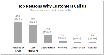
You can change data labels and point them to different cells using this little trick.
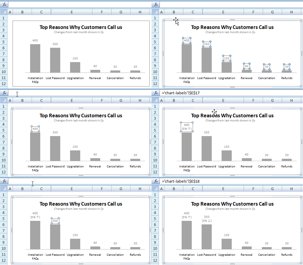
 First add data labels to the chart (Layout Ribbon > Data Labels)
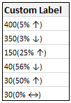
- Define the new data label values in a bunch of cells, like this:
- Now, click on any data label. This will select “all” data labels. Now click once again. At this point excel will select only one data label.
- Go to Formula bar, press = and point to the cell where the data label for that chart data point is defined.
- Repeat the process for all other data labels, one after another. See the screencast.
Points to note:
- This approach works for one data label at a time. So if you have a large chart, you are in for a lot of clicks and manic mouse maneuvering.
- That brings us to Rob Bovey’s Chart Labeler Excel Add-in. This free tool can automate the whole custom chart labeling for you.
- If you want more formatting options, consider adding text boxes and point them to cells instead. See the smart chart legends post.
Share your Chart Formatting Tricks:
What are your favorite chart formatting tricks? My favorite tricks are using text boxes to add rich formatting to charts (example here) and messing with fonts and colors (some rules here).
What about you?
Recently in Charting:


65 Responses
I sometime use a dummy data series plotted on the secondary axis. You can then set the secondary category labels to use the range with the custom labels text.
Apply Category data labels to the dummy series.
Personally, I think this is a great tip. I like the idea of automating the process, although I’m always hesitant to use “add-ons.” It seems like it would be a fairly straightforward VBA project. In fact, you could probably use VBA to automatically make the labels themselves, so you didn’t need the source cells. I’ll look into this the next time I’m needing custom labels.
Bob Bovey’s Chart Labeler Add-in (linked above) works like a charm. I needed to add alpha labels to the bubbles in a bubble chart and it gives me exactly what I needed.
You can use the same trick to relabel axes – this is great if you’re using the offset formula with a dropdown to create a dynamic chart = just change the axes title as well using an offset.
I know this is but an excel trick, but …
I think I’d rather see two charts: one with the numbers as displayed and another with the %change between the 2 months. Better yet would be to display the last several months as line charts. Change always needs to be seen in the context of history.
hi guys, this works if you have a single series.
what about stacked bar (multiple series)?
e.g. i have March and April series stacked-bar chart. i’d like to label the TOTAL of both months, but the data label should be [outside-end] of April’s bar.
[March]-[April]-[data label of the total for Mar+Apr]
normal labelling dont offer [outside-end] data labelling. Rob Bovey’s Chart Labeler also doesnt offer this.
any ideas?
@David: You can add a dummy series to the stacked bar and stacked it on top of the last month. Now, make the dummy series transparent (no fill, no border) and set labels to it (at inside end). Use the technique in this post to customize labels and you should be good to go.
dear I got your point, but it will show label at x- axis only , how to raise that to the primary series data level , that height just next to the primary series values.
ahhh yes, that’s what I’m thinking of too 😉
cheers!
Brill tip….as usual!
@David,
you can also calculate the totals in your data, then add the total series to the chart, move it to the secondary Y axis, change the chart type to a column (not stacked column) chart. Then add data labels for the total series, which you can now place to the outside end of the columns. Finally format the total series to no fill and no line to make it invisible.
cheers, teylyn
@David… Teylyns tip is better than mine. With that you dont have to fix the axis scales.
@Andy & @Alex… good additions 🙂
@Bill: Of course using separate charts is even better. My intention is to show the trick related to chart label customization.
@Teylyn… Excellent. Here is your donut 🙂
thx teylyn 😉
chandoo, i prefer adding another dummy series; BUT with small value (and clickable!) so that it won’t force change the axis scale 😉
anyhow, both methods have its merits 😀
Dont know if anybody has come across this before, but I’ve been using it (well, my own slightly modified version of the code) to add labels to charts and it works very very well
http://support.microsoft.com/kb/914813
-Dan
chandoo, how do u ‘break’ the data labels into 2 lines (like those displayed on the chart)?
e.g. 400 (5%) ==> 400 (5%)
David,
You can press Alt+Enter after 400 to get data lables in 2 lines.
How do you do to brake labels into 2 lines if the link is a concatenate? Alt+Enter doesn’t work in this case… Any ideas? Thanks.
Got it!!!
I might be of help for someone, so here it goes:
Just place CHAR(10) were you want the break and that’s it!
E.g.: =A1&CHAR(10)&A2
My full formula to keep format is:
=TEXT(A1,”0,000″)&CHAR(10)&”(“&TEXT(A2,”0.0%”)&”)”, were A1 is my amount and A2 my growth %.
Thanks Chandoo for such a wonderful tip….
Please guide me How to make arrow like ” Custom Label” table.
Thanks
wow, that works Pipo 😉
thanx!
Thanks dude – making my charts look good – management thinks im the bomb!!
really very useful…Thanks a lot….
So, now that there are custom data labels, is there any way to change the text justification? All I ever see is centered text but I would like to have mine left justified. Whatever the formatting is in the linked cell doesn’t get reflected in the chart. In your example it works OK since there is a number (short length) and then a percent change (longer length). The centering looks OK there. I am working on a time line and would like the labels in more of a list format rather than centered. Thanks.
Hello Chandoo.. Great tip.. Would i be able to color the arrow using formula itself??
Hi Chandoo,
didn’t know that we can do that ^^. Out of the topic. is it possible to make the axis label interactive as well. We can change the data through name range but I can seem to find the answer for axis label. I am trying to make interactive bar chart with different number of data and different axis label (name of region for example).
@Fitriadi
Put the text in A1 you want as your Axis label
Select the Axis Label you want to change
With it selected click in the formula Bar at the top of the screen and type =A1
Select with the Tick to the left of the formula bar
Change reference to suit
@Hui
Hi Hui, thanks for the quick reply. But I think what you mean is axis title, because i cant seem to click on the formula bar when i click on the axis label. I did able to do it with the axis title though.
I have a chart with two axis on the X axis I have the date on the two Y axis i have bar and line data. The Line data shows from 30 to 70 in increments of 10. I want the 70 to show a label £ without putting in a text box eg £70 and none of the other figures will have the £ sign. Is there a formula or a quick way in Excel 2003 to do this.
Many thnaks
@John
Select the X-Axis you want to format
Right Click, Format Axis
Add a Custom Number format of “£”0
Thanks Hui but that changes all the values to have the pound sign I only want one value to show with the £ sign. And these values are on the y axis. There are two y axis.
You can’t format a single entry or component of an axis text
Easiest way would be to add a text box to the chart
“Formula used to create £ symbol on secondary scale (i.e. not text box)”
This is part of the test I have to do Hui so you must be able to do it otherwise it wouldn’t be part of the test.
I am at a complete loss on this one I have tried all the methods you have described.
John
@John
Select the X-Axis you want to format
Right Click, Format Axis
use the following Custom Number format
[<70]"";[=70]"£"0;;
Brilliant I had to ammend slightly but spot on.
[<70]general;[=70]£0;;
Thank you so much Hui.
John
What great info! This and other tips on this site are awesome. Thanks Chandoo!
This is awesome! Saved my day
Has someone figured out how to do this in VBA code? This is exactly what I need.
How do I format labels in a scatter plot with over 200 labels to change. Is there no way of creating a column with the labels you want so that excel automatically includes these labels instead of the ‘series labels’
Hi Chandoo
I used the XY Labeler and it worked for me.
Thanks
Vipul
It’s Very Helpful to me ~ Thank A lot.
Hi,
Great info!! I want to know if it possible to hide a specific data label except when the cursor is in the data.
For instance, I have a lot of wells plotted in a XY chart with a map as a background, the x and y are the coordinates of each well. However, when I want to know a specific well in the chart is so hard to find it, I need to check the coordinates in the chart and then find to which well correspond those coordinates. If I put all the well label the chart looks messy.
What do you recommend me??
Thank you in advance
@Itzel
I would add another series which highlighted a specific well
Add a Drop Down which lists all the wells
Using the Cell Link from the drop down, Retrieve the X & Y co-ords for the well
Plot the well as a Marker using a new series on the chart
It may be worth while you uploading a copy of the file, Refer: http://chandoo.org/forums/topic/posting-a-sample-workbook
I’ve used the tip from the tutorial and it works great until now. I have to move the entire xlxs file from my computer onto a flash drive to get it to my computer at work but I loose he Data Labels when I move my project. It just says cell reference instead.
Anyone know how to move my file and still keep the Data Labels?
Thank you in advance!
This should not be the case. Did you make sure the cells to which data labels refer to contain the data?
Well yes. To clarify, everything works perfect on my computer. And all the cells witch the data labels refers to contains data and there in the same workbook as the chart. Just on a different sheet. Then I make a copy of the file, put it on a flash drive and even tjen, when I open the file from the flash drive on the same computer everything works perfect. But when I put my flash drive in another computer (I’ve tried several) the data labels doesn’t refesh! All cells looks the same. The chart works just fine. Text box’s within the chart aswell. Just not the data labels. And I have somewhere between 150 and 200 of hem. I don’t want to update all of the manually everytime I move the file. Please help.
What if you use another means to transfer the file (say email or file sharing service)?
Chandoo, thank you for your wonderful site – I really like the way you present info!
Is it possible to make the custom data label table dynamic, ie up/down/sideways arrow depending on changing data? I don’t want to use any add-ins.
Thank you this has helped a ton and saved me time 🙂
Thanks, great tip.
One problem, I cant seem to conditionally format the data labels now. EG, Red font for minus %, which I can to in a ‘normal’ data label.
Any ideas how to get around this?
@JohnH
Try: [Black]0.0,[Red]-0.0,0.0
@Hui
Yes this is what I would normally use. But seemingly with the ‘custom data labels’ this doesn’t seem to work. I guess it makes sense as with the custom labelling, you could be putting anything in as a label.
I’ve worked out a workaround now anyway, its a bit long winded, but it works!
Cheers
Hi,
I have a bar chart that shows actual performance against targets (overlapping bars) and what I would like is for the data label to show the % of actual vs target. I can get a column in my pivot that shows this but don’t know how to have the label from another data set showing.
The graph is linked to a pivot with a slicer which makes it even harder to pull together.
Any ideas?
Thanks!
Anna
Any ideas>?
This VBa code changes labels one by one for you:
Sub GraphsShowSeriesName()
‘activates datalabels of a chart and changes ALL
‘of them from the default showvalues, to Seriesname one by one.
ActiveChart.ApplyDataLabels
Dim item As Variant
For Each item In ActiveChart.SeriesCollection
item.DataLabels.ShowSeriesName = True
item.DataLabels.ShowValue = False
Next item
End Sub
Thank you! This was the first article when I searched.
Thank you! Worked perfect
In Excel 2016, after generating a data label,
> double click data label
> Label options
> Label contains/Value From Cells
Here you could select the data range of custom data label.
One problem I have found – I have a 10 bar chart with the 10 bars individually linked to labels that sit in a grid alongside the source data.
If I decide to hide or group together rows, the labels go out of sync.
For example, If I group row 5 the charge removes the bar for that set of data but the label that was linking to bar 5 is now assigned to the new 5th bar, which was actually my 6th row of data. Bars 7, 8, 9 and 10 are also now showing the wrong labels.
I don’t know of a solution, but in my case the labels were numeric values so I just changed to a stacked bar chart and added a clear stack above the data with the values plotted as data.
Hi I am preparing a X-Y scatter chart. Now when i hover over the scatter points, a hover label appears which shows the values corresponding to the X,Y values. Now I also want that hover label to display additional name mentioned against each Y values in the column adjacent to the Y series column. I had done all the research but not bale to find any solution….can anyone help.
@Ankit
You could consider trying a Bubble Chart
First I realise that this post is not an exact follow-on from the main topic, but now I think what I am asking for is another type of custom labels, and this thread is as close as I can find, so here goes….
Can I request some help with charts?
I Have 4 columns of data to plot. Sounds easy, right?
This is the only page in a new spreadsheet, created from new, in Win Pro 2010, excel 2010.
Cols C & D are values (hard coded, Number format).
Col B is all null except for “1” in each cell next to the labels, as a helper series, iaw a web forum fix.
Col A is x axis labels (hard coded, no spaces in strings, text format), with null cells in between.
The labels are every 4 or 5 rows apart with null in between, marking month ends, the data columns are readings taken each week.
Y axis is automatic, and works fine.
1050 rows of data for all columns (i.e. 20 years of trend data, and growing).
The Chart I have created (type thin line with tick markers) WILL NOT display x axis labels associated with more than 150 rows of data.
(Noting 150/4=~ 38 labels initially chart ok, out of 1050/4=~ 263 total months labels in column A.)
It does chart all 1050 rows of data values in Y at all times.
I change the charted data range to 160 or more rows of data (155 to all 1050) and suddenly the labels become random.
It will display labels 1, 4 , 6 , 7, 9 , 10, 15, and miss all labels in between and all after 100 data rows.
I revert to 150 data lines plotted, it goes back to first 38 labels ok.
Repeat to 160+ rows plotted, random again, only with a new random selection of labels displayed. All others are missing.
So the chart is now largely meaningless, since you can not tell how fast the readings are increasing.
I have played around with numbers of rows (using 100 to 1050), chart types line, scatter, and ribbon, even cone – same happens when I change the number of data rows in all types.
I have played with the format of the chart in every way I can find a control for, including drag/expanding 165 row ticks out to 3 times A3 page size to make 2cm gaps between labels, does not reinstate the missing labels.
Is this a known bug with later versions of excel ?
(like finding the hard way cells now only hold 255 characters, so losing half your clients comments ! )
Is there a work around?
(note the same data set in my old home XP excel charts this fine in every way)(and on the first go)(copied hard data from old XP version)
Thank you, Chandoo.
Best Regards, M
Hello! Quick question that’s entirely off topic. Do
you know how to make your site mobile friendly? My website looks weird
when browsing from my iphone. I’m trying to find a template or plugin that
might be able to resolve this problem. If you have any suggestions, please
share. With thanks!
Hi in my Chart data labels reflecting for (slicer) person A and I am changing in B it’s not reflecting please help me to identify the error and make it correct