ABC Inventory Analysis using Excel

ABC analysis is a popular technique to understand and categorize inventories. Imagine you are handling inventory at a plant that manufactures high-end super expensive cars. Each car requires several parts (4,693 to be exact) to assemble. Some of these parts are very costly (say few thousand dollars per part), while others are cheap (50 cents per part). So how do you make sure that your inventory tracking efforts are optimized so that you waste less time on 50 cent parts & spend more time on costly ones?

This is where ABC analysis helps.

We group the parts in to 3 classes.

• Class A: High cost items. Very tight control & tracking.
• Class B: Medium cost items. Tight control & moderate tracking.
• Class C: Low cost items. No or little control & tracking.

Given a list of items (part numbers, unit costs & number of units needed for assembly), how do we automatically figure which class each item belongs to?

And how do we generate below ABC analysis chart from it?

That is what we are going to learn. So grab your inventory and follow along.
(related: ABC Analysis page on Wikipedia)

ABC Analysis using Excel – Step by step tutorial

1. Arrange the inventory data in Excel

Pull all the inventory (or parts) data in to Excel. Your data should have at least these columns.

• Part Name
• Unit cost
• # of units (if this is blank, just type 1 in all rows)

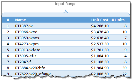
Once the data is in Excel, turn it in to a table by pressing CTRL+T. Lets call our data as inventory. You can set the table name from Design tab.

(Related: Introduction to Excel Tables)

2. Calculate extra columns needed for ABC classification

Now comes the fun part. Crunching the inventory data with formulas. Yummy!

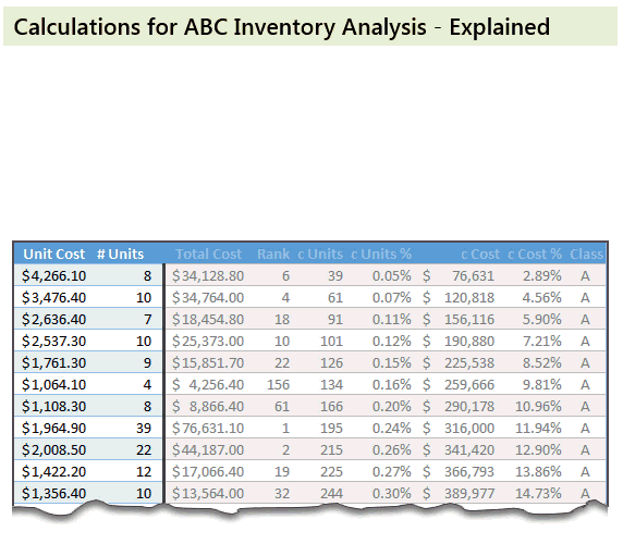
Total Cost: This is just a multiplication of unit cost & # of units columns

Rank: We need to figure out what rank each total cost is (in the total cost column). We can use RANK formula for this.

=RANK([@[Total Cost]],[Total Cost],0) will tell us the rank for each total cost.

Cumulative Units: Once we know the rank of each item, next we need to figure out how many total units are needed for items ranked less or equal.

For example, The number (#) of the third part (PT3959-waes) is 3. Cumulative units for this is 91. This means, 91 is the total number of units for first three ranked parts (parts # 8, 9, and 16).

The formula for this is, =SUMIFS(['# Units],[Rank],"<="&[@['#]])

Remember, [@[‘#]] refers to running numbers (1,2,3….4692,4693)

Cumulative Units %: This is a percentage of cumulative units in total. The formula is simply,

=[@[c Units]]/MAX([c Units])

[Related: using structural references in Excel – video]

Cumulative Cost & Cumulative Cost %:

These are similar calculations (instead of units, we calculate cost)

Explanation of these calculations:

See below animation to understand how the numbers are crunched.

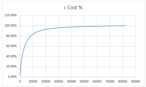
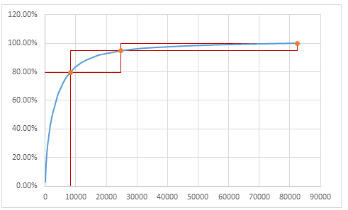
3. Create Inventory Distribution Chart

Select cumulative units & cumulative cost % columns and create an XY chart. Make sure cumulative units is on horizontal (X) axis and cumulative cost % is on vertical (Y) axis.

Our curve should look something like this.

4. Set up ABC classification thresholds

Now we need to decide what is the threshold for classes A,B & C.

For most situations, Class A tends to be top 10% of the items.

Class B would be next 20%

Class C would be the last 70%.

But these numbers may change depending on your industry, manufacturing settings.

Lets say, some where in our spreadsheet, user has defined the thresholds for the classes in a range like this:

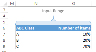
So $O$7:$O$9 contains the thresholds.

Next to this range, calculate additional numbers (for plotting A, B & C markers and boxes) like this:

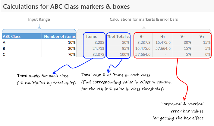
Examine the download file for exact formulas.

5. Add the ABC items & % total cost columns to chart

Add the extra data to the chart (by right clicking on chart and going to select data box & clicking “Add” button).

Once the new series is added, make sure you format it as markers only so that we get something like this.

6. Add Error bars to the ABC markers to get boxes

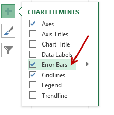This step involves adding error bars to ABC marker series and customizing them.

In Excel 2013: Add error bars by clicking on the + button next to chart

In earlier versions: Do this from layout ribbon

Once error bars are added, customize them (select and press CTRL+1). Set error amount to Custom and select the calculated error values as shown below.

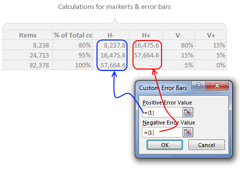
Once added, format the error bars to show no cap and change line color to something pleasant.

Now we have boxes on the chart.

7. Clean up the chart, add labels & titles

This is where get creative. After some clean up, we can arrive at something like this.

Download ABC Inventory Analysis Template Workbook

Click here to download ABC Inventory Analysis workbook. It contains sample data & chart. Examine the formulas & chart settings to learn more. Or if you are in a hurry, replace the sample data with your inventory details and get instant results.

Do you use ABC analysis for inventory tracking & control?

I will be honest. I have never worked as inventory controller in a super-car manufacturing plant. That said, I run a business and we do have inventory. Not physical but digital inventory. So I often use analysis like ABC or pareto to quickly figure out where I should focus my efforts.

What about you? Do you use techniques like ABC analysis to narrow down to a few items that matter most? How do you do it in Excel? Please share your tips & experiences using comments.

Add few more techniques to your inventory

Feeling low on your Excel skills inventory? Stock up with below goodies.

• Pareto Analysis in Excel – How to & tutorial
• Analyzing competition using charts – case study
• Track employee vacations & productivity [dashboard & tutorial]
• Track annual goals & achievements