
Back when I was working as a project lead, everyday my project manager would ask me the same question.
“Chandoo, whats the progress?”
He was so punctual about it, even on days when our coffee machine wasn’t working.
As you can see, tracking progress is an obsession we all have. At this very moment, if you pay close attention, you can hear mouse clicks of thousands of analysts and managers all over the world making project progress charts.

So today, lets talk about best charts to show % progress against a goal.
Please download example file and keep it handy while reading the rest of this tutorial.
Data for these charts
For all these charts, we will use below data:
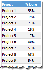
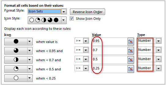
Chart #1: Conditional Formatting Icons + % values
This is my all time favorite. It is very easy to implement and works really well.
All you have to do is,
- Select the % completion data
- Go to Home > Conditional Formatting > Icon sets
- Select 3 traffic lights
- Edit the rule as shown below:
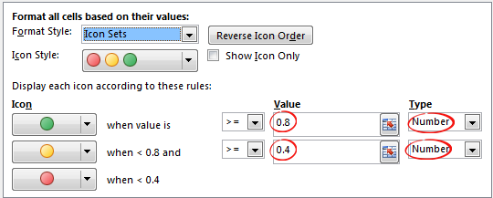
- Done!
Why you should use this?
- Very easy to set up.
- Scalable. Works the same when you have 20 or 200 or 2000 items to track.
- Looks great
Keep in mind:
- The traffic lights in Excel are not great for color-blind people.
- The traffic lights do not look good when printed in black-and-white (or gray scale)
Related: Never show simple numbers in your dashboards
Chart #2: Conditional Formatting Data Bars
Another easy and quick answer.
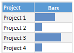
- Select % completion data
- Go to Home > Conditional Formatting > Data bars
- Select Solid Fill if available.
- Done!
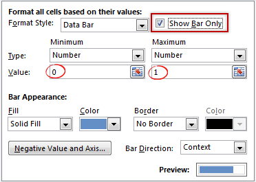
- Extra step: Adjust maximum bar size to 100% so that you can see relative progress better.
Why you should use this?
- Very easy to set up.
- Scalable. Works the same when you have 20 or 200 or 2000 items to track.
Keep in mind:
- By default the maximum value in your data takes 100% of the cell width. So make sure you set this to 100% for better depiction of progress.
Chart #3: In-cell bar charts
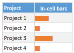
If for some reason you cannot use databars, then rely on in-cell bar charts. These are simple to setup and works great in many situations where conditional formatting may not be an option.
- Assuming your % data is in A1,
- In adjacent cell (B1), write = REPT(“|”, A1*100)
- You will get a lot of pipe symbols | in this cell.
- Select the cell and change font to Playbill
- Adjust font size and color if needed.
- Done!
Why you should use this?
- Very easy to set up.
- Scalable. Works the same when you have 20 or 200 or 2000 items to track.
- Can be handy when making dashboards or reports (where conditional formatting may have limitations)
Keep in mind:
- The font & size has impact on how in-cell chart is displayed. Use either Playbill or Script fonts.
Chart #4: Pies
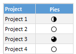
Conditional formatting pie charts are a simple alternative to show % progress data.
The process is same as traffic light icons. Make sure you adjust pie icon settings as per your taste.
Why you should use this?
- Very easy to set up.
- Scalable. Works the same when you have 20 or 200 or 2000 items to track.
Keep in mind:
- Pie chart icons have only 5 stops. So they are not really pies.
- Not everyone likes pie charts. Make sure your boss / customers dig them.
Chart #5: Color scales or heat maps
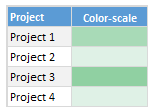
When you have a lot of items to track, your focus is really on which items are lagging (or leading). In such cases, a color scale (also known as heatmap) can work very well. It colors cells based on their value. For example, the darker a cell color is, the more that particular project is done and vice-versa.
Why you should use this?
- Very easy to set up.
- Scalable. Works the same when you have 20 or 200 or 2000 items to track.
Keep in mind:
- Make sure the color starting & end points are well contrasted. Else the color scale looks bland.
- By default color scales show the values too. To hide them use ;;; custom cell formatting code (how to).
Chart #6: Thermometer charts
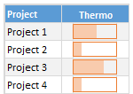
This is my favorite technique. It works very well for data like this.
Tutorial on how to create thermometer charts.
Why you should use this?
- Easy to understand
- Scalable. Works the same when you have 20 or 200 or 2000 items to track.
Keep in mind:
- If any value is more than 100% the chart may not explain it properly.
- Make sure the axis min & max are set to 0 and 1 respectively.
- You need a dummy column with 100% in it to show outline of thermometer.
Download Examples
Click here to download example workbook. It contains all these charts.
Special bonus for you:
As a bonus, the download workbook also has 5 step tracker to make you awesome in Excel. Go ahead and download now.
What is your favorite chart to show % progress?
My most favorite chart is thermometer. The next is traffic light icon-set.
What about you? Which of these 6 is your favorite? Please share your chart in the chart. If you use something else altogether, please tell me. I am eager to learn from you.
More on comparison charts

Just like my project manager, I am sure your manager too loves tracking & comparison. If so, please go thru below articles to learn few more tricks to impress her.
- Us vs. Them – compare one value with many using interactive chart
- Best charts to compare budget with actual values
- Indicating lower & upper bounds on a chart
- Customer service dashboard – a case study in comparison
- Exploring Flu trends in excel chart – a case study in heat maps for comparison
Now if you excuse me, I have to report to my new project manager: my wife. She is asking me about the progress of taking down Christmas lights. And I am still at 9%.


20 Responses to “Simulating Dice throws – the correct way to do it in excel”
You have an interesting point, but the bell curve theory is nonsense. Certainly it is not what you would want, even if it were true.
Alpha Bravo - Although not a distribution curve in the strict sense, is does reflect the actual results of throwing two physical dice.
And reflects the following . .
There is 1 way of throwing a total of 2
There are 2 ways of throwing a total of 3
There are 3 ways of throwing a total of 4
There are 4 ways of throwing a total of 5
There are 5 ways of throwing a total of 6
There are 6 ways of throwing a total of 7
There are 5 ways of throwing a total of 8
There are 4 ways of throwing a total of 9
There are 3 ways of throwing a total of 10
There are 2 ways of throwing a total of 11
There is 1 way of throwing a total of 12
@alpha bravo ... welcome... 🙂
either your comment or your dice is loaded 😉
I am afraid the distribution shown in the right graph is what you get when you throw a pair of dice in real world. As Karl already explained, it is not random behavior you see when you try to combine 2 random events (individual dice throws), but more of order due to how things work.
@Karl, thanks 🙂
When simulating a coin toss, the ROUND function you used is appropriate. However, your die simulation formula should use INT instead of ROUND:
=INT(RAND()*6)+1
Otherwise, the rounding causes half of each number's predictions to be applied to the next higher number. Also, you'd get a count for 7, which isn't possible in a die.
To illustrate, I set up 1200 trials of each formula in a worksheet and counted the results. The image here shows the table and a histogram of results:
http://peltiertech.com/WordPress/wp-content/img200808/RandonDieTrials.png
@Jon: thanks for pointing this out. You are absolutely right. INT() is what I should I have used instead of ROUND() as it reduces the possibility of having either 1 or 6 by almost half that of having other numbers.
this is such a good thing to learn, helps me a lot in my future simulations.
Btw, the actual graphs I have shown were plotted based on randbetween() and not from rand()*6, so they still hold good.
Updating the post to include your comments as it helps everyone to know this.
By the way, the distribution is not a Gaussian distribution, as Karl points out. However, when you add the simulations of many dice together (i.e., ten throws), the overall results will approximate a Gaussian distribution. If my feeble memory serves me, this is the Central Limit Theorem.
@Jon, that is right, you have to nearly throw infinite number of dice and add their face counts to get a perfect bell curve or Gaussian distribution, but as the central limit theorem suggests, our curve should roughly look like a bell curve... 🙂
[...] posts on games & excel that you may enjoy: Simulating Dice throws in Excel Generate and Print Bingo / Housie tickets using this excel Understanding Monopoly Board [...]
[...] Correct way to simulate dice throws in excel [...]
[...] Simulate dice throws in excel [...]
I'm afraid to say that this is a badly stated and ambiguous post, which is likely to cause errors and misunderstanding.
Aside from the initial use of round() instead of int(),.. (you've since corrected), you made several crucial mistakes by not accurately and unambiguously stating the details.
Firstly, you said:
"this little function generates a random fraction between 0 and 1"
Correctly stated this should be:
"this little function generates a random fraction F where 0 <= F < 1".
Secondly, I guess because you were a little fuzzy about the exact range of values returned by rand(), you have then been just as ambiguous in stating:
"I usually write int(rand()*12)+1 if I need a random number between 0 to 12".
(that implies 13 integers, not 12)
Your formula, does not return 13 integers between 0 to 12.
It returns 12 integers between 1 and 12 (inclusive).
-- As rand() returns a random fraction F where 0 <= F < 1, you can obviously can only get integers between 1 and 12 (inclusive) from your formula as stated above, but clearly not zero.
If you had said either:
"I usually write int(rand()*12) if I need a random number between 0 to 11 (inclusive)",
or:
"I usually write int(rand()*12)+1 if I need a random number between 1 to 12 (inclusive)"
then you would have been correct.
Unfortunately, you FAIL! -- repeat 5th grade please!
Your Fifth Grade Maths Teacher
Idk if I'm on the right forum for this or how soon one can reply, but I'm working on a test using Excel and I have a table set up to get all my answers from BUT I need to generate 10,000 answers from this one table. Every time, I try to do this I get 10,000 duplicate answers. I know there has to be some simple command I have left out or not used at all, any help would be extremely helpful! (And I already have the dice figured out lol)
Roll 4Dice with 20Sides (4D20) if the total < 20 add the sum of a rerolled 2D20. What is the average total over 10,000 turns? (Short and sweet)
Like I said when I try to simulate 10,000turns I just get "67" 10,000times -_- help please! 😀
@Justin
This is a good example to use for basic simulation
have a look at the file I have posted at:
https://rapidshare.com/files/1257689536/4_Dice.xlsx
It uses a variable size dice which you set
Has 4 Dice
Throws them 10,000 times
If Total per roll < 20 uses the sum of 2 extra dice Adds up the scores Averages the results You can read more about how it was constructed by reading this post: http://chandoo.org/wp/2010/05/06/data-tables-monte-carlo-simulations-in-excel-a-comprehensive-guide/
Oh derp, i fell for this trap too, thinking i was makeing a good dice roll simulation.. instead of just got an average of everything 😛
Noteably This dice trow simulate page is kinda important, as most roleplay dice games were hard.. i mean, a crit failure or crit hit (rolling double 1's or double 6's) in a a game for example dungeons and dragons, if you dont do the roll each induvidual dice, then theres a higher chance of scoreing a crit hit or a crit failure on attacking..
I've been working on this for awhile. So here's a few issues I've come across and solved.
#1. round() does work, but you add 0.5 as the constant, not 1.
trunc() and int() give you the same distributions as round() when you use the constant 1, so among the three functions they are all equally fair as long as you remember what you're doing when you use one rather than the other. I've proven it with a rough mathematical proof -- I say rough only because I'm not a proper mathematician.
In short, depending on the function (s is the number of sides, and R stands in for RAND() ):
round(f), where f = sR + 0.5
trunc(f), where f = sR + 1
int(f), where f = sR + 1
will all give you the same distribution, meaning that between the three functions they are fair and none favors something more than the others. However...
#2. None of the above gets you around the uneven distribution of possible outcomes of primes not found in the factorization of the base being used (base-10, since we're using decimal; and the prime factorization of 10 is 2 and 5).
With a 10-sided die, where your equation would be
=ROUND(6*RAND()+0.5)
Your distribution of possible values is even across all ten possibilities.
However, if you use the most basic die, a 6-sided die, the distributions favor some rolls over others. Let's assume your random number can only generate down to the thousandths (0.000 ? R ? 0.999). The distribution of possible outcomes of your function are:
1: 167
2: 167
3: 166
4: 167
5: 167
6: 166
So 4 and 6 are always under-represented in the distribution by 1 less than their compatriots. This is true no matter how many decimals you allow, though the distribution gets closer and closer to equal the further towards infinite decimal places you go.
This carries over to all die whose numbers of sides do not factor down to a prime factorization of some exponential values of 2 and 5.
So, then, how can we fix this one, tiny issue in a practical manner that doesn't make our heads hurt or put unnecessary strain on the computer?
Real quick addendum to the above:
Obviously when I put the equation after the example of the 10-sided die, I meant to put a 10*RAND() instead of a 6*RAND(). Oops!
Also, where I have 0.000 ? R ? 0.999, the ?'s are supposed to be less-than-or-equal-to signs but the comments didn't like that. Oh well.
How do you keep adding up the total? I would like to have a cell which keeps adding up the total sum of the two dices, even after a new number is generated in the cells when you refresh or generate new numbers.
So, how do you simulate rolling 12 dice? Do you write int(rand()*6) 12 times?
Is there a simpler way of simulating n dice in Excel?
I've run this code in VBA
Sub generate()
Application.ScreenUpdating = False
Application.Calculation = False
Dim app, i As Long
Set app = Application.WorksheetFunction
For i = 3 To 10002
Cells(i, 3).Value = i - 2
Cells(i, 4).Value = app.RandBetween(2, 12)
Cells(i, 5).Value = app.RandBetween(1, 6) + app.RandBetween(1, 6)
Next
Application.ScreenUpdating = True
Application.Calculation = True
End Sub
But I get the same distribution for both columns 4 and 5
Why ?
@Mohammed
I would expect to get the same distribution as you have effectively used the same function