
A while ago (well more than 3 years ago), I wrote about an array formula based technique to check if a list of values have any duplicates in them.
Today, lets learn a simpler formula to check if a list has duplicate numbers.
Assuming you have some numbers in a range B4:B10 as shown below,
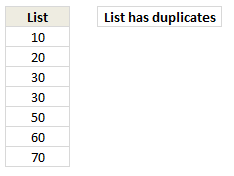
You can use COUNTIF & MODE formulas to check if the list has any duplicates, like this:
=IF(COUNTIF($B$4:$B$10,MODE($B$4:$B$10))>1, "List has duplicates", "No duplicates")
How does it work?
MODE formula gives us the most frequently occurring number in a list. Then, we use COUNTIF to see how many times this number occurs in a list.
In a list with no duplicates mode value occurs only 1 time. If a list has duplicate numbers, then count of mode would be more than 1. That is what the IF formula checks for and then prints appropriate message.
See this example:
[Embedded Excel, if you can not see it, click here]
Play with below embedded Excel file to understand the technique. You can modify numbers or formula.
Or Download this Example
Click here to download the example workbook and play with it.
How do you check if a list has duplicates?
For text values, I use the array formula technique described here. For numeric values, I prefer MODE + COUNTIF combination because it is easy to write & explain.
What about you? How do you check if a list has duplicates? Which formulas do you use? Please share your techniques using comments.
More on Duplicates & Unique values
If we analyze the time an analyst spends on various things, we would realize,
- 30% of time cleaning data (removing duplicates etc.)
- 30% of time actual analysis
- 30% of time drinking coffee
- 10% of time actual presentation
On a more serious note, if you want to learn various techniques to deal with duplicate values, read on:
- Extracting unique values from a list in Excel using formulas
- Extracting unique values from a list using Pivot tables
- Count the number of values in a list (excluding duplicates)
- Quickly compare 2 lists and check for duplicates
- Removing duplicate values quickly
- Avoiding duplicate data entry using Data Validation


17 Responses to “Custom Number Formats – Colors”
You are right, Chandoo. I was playing with the colour numbers last week and some of them don't appear different from each other. Others are totally different from yours.
@Duncan
Each version of Excel, post 2003, renders colors slightly differently
Different language versions may also have different default color palettes
Hello in french
excel 2010
colo1 = couleur1 = black
[couleur1]; [couleur2]; etc..
@Hui, thank you very much again for this great post.
However - under Excel 2007, Hungarian version your solution does not work with color names. I've tried both English and Hungarian names, but drops an error message "not valid formats"
Do you have any idea how to solve this issue?
thanks in advance
@Andras
Without a Hungarian version of Excel 2003 I don't think I can assist
Have you tried using the colour numbers? I couldn't get the names to work (despite using an english version of excel). but it did work with the numbers though. I left out the "u" and was easily able to produce burgundy using [color9]
Here a possible solution: find an English version of Excel, write there the formats using English names, then open the file in the Hungarian version and see the translation.
In Excel 2007 I can't get the colour names to work e.g Sea Green but the numbers do e.g color3 - colour3 does not work so I must bow to the country that has stolen my language (ha ha!)
Hey chandoo, nice Tip!
Wouldn't be easier just apply some conditional formatting for negative numbers and another for positive numbers? Or there's some cases that you can't do that?
Unfortunately the TEXT function doesn't color the cell as number formatting does.
Hi Hui,
Great post Sir, love the new way of formatting with color numbers.
I am using 2007, and it leads me to the last color number 56.
Thanks Hui.
[…] explains how to set up custom number formats with a wide array of […]
Thanks Hui - works a treat!
Thank you, very helpful.
Trying to figure out if it is possible to apply color only to a part of the cell?
E.g. I have a value formatted as Accounting with a currency symbol.
Those I find somewhat distracting though necessary. If I could make them less obtrusive by coloring them gray while the number would stay black, that would be great. Tried tinkering with the format string, but didn't get the desired result. Single color for complete cell value works, but coloring just part of it could not be achieved. Maybe somebody managed that?
Exactly what I was looking for - thank you!
colour in the Australian doesn't work - we have to go American and no problem.
I always thought is was 56 colours notice you have 57. Cool.
thanks
Analir Pisani
Customised Microsoft Office Training Specialist
Sydney - Australia
http://www.azsolutions.com.au
Thank You!