
The other day, I got a text message (SMS) from one of our readers. It read,

So today, let us learn a very easy trick to select random sample from your data.
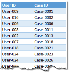
Lets take a look at the data
Since the text message has no actual data, I made up this.
Now, if you just want to select any 10 (or x number of) random items from this list, then your job would very simple.
- Shuffle (or randomly arrange) this list
- Just pick first 10 items
But our problem is to get 2 random samples per user.
Selecting random samples from data
Follow below steps.
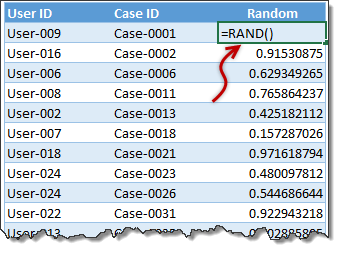
- Add an extra column and fill it with =RAND() formula. This generates random fraction between 0 and 1.
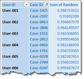
- Create a pivot table from this data (tutorial: How to create a pivot table?)
- Add User ID & Case ID as Row labels and Random as value field.

- Click on the filter icon on Case ID column, choose Value filter > Top 10
- Filter for top 2 random values. (related: Filter top 10 values in pivot tables – how to?)

- Adjust report layout (Table layout, no sub-totals, no grand totals)

- Done!
To see new samples
Just select any cell in the pivot table, press ALT+F5. Your pivot table will be refreshed and you get new samples.
That is just easy and awesome!
Download Example Workbook
Click here to download the example file. Refresh the pivot table (ALT+F5) to see fresh samples.
Do you sample your data?
Drawing samples, running experiments, analyzing results are life breath for many businesses. As business data is growing, these analytical skills are becoming important.
How do you draw samples? What techniques you use when analyzing the data? Please share your stories, experiences & tips using comments.
A sample of our awesome collection of Excel tips
Here is a tiny sample of our awesome Excel tips. Don’t hold back, take them all, and more.
- Introduction to Pivot Tables
- How to shuffle a list of values in Excel
- How to shuffle a list using Formulas
- How to generate a random date, phone number
- Introduction to Excel’s random functions
- Case study: Generating housie (bingo) number cards using Excel
- Game: Simulating Deal or No Deal game in Excel


One Response to “Excel Tips Submitted by You [Part 4]”
ctl+d
copy the up cell