
Today, lets understand how to use Calculated items feature in Pivot tables. We will use a practical problem many of us face to learn this feature – ie calculating conversion ratio from a list of sales calls.
This is inspired from a question posted by Nicki in our forums,
I have a spreadsheet source data full of sales enquiries which have the Status – Lost, Booked or Pending. Each sales enquiry relates to a particular location. I have created a pivot table which counts the enquiries and displays them with the Locations in rows and the Status in the columns. I have got a row total showing the total number of sales enquiries for each location. I also want my table display the sales conversion number, ie the booked enquiries as a % of the total enquiries. How do I do this?
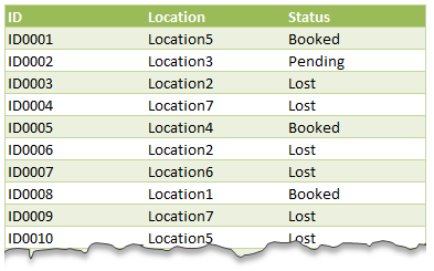
A look at the data
Lets say, you have some data like this and you want to understand what is the conversion ratio by location.
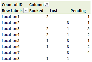
Setup a pivot table
The first step is to just create a pivot table from this data. Put locations in row labels area, status in column labels are and ID in values area. Now you will have a count of items for each status in each location. Something like this:
Add a calculated item to get conversion ratio
Now we want to calculate how much percentage is “booked” status items in all items for a location. To do this,
- Select any column label item in the pivot table.
- Click on Pivot Options > Fields, Items & Sets > Calculated item

- Give your calculated item a suitable name like Conv. %
- Write the formula = Booked / (Booked + Pending + Lost)
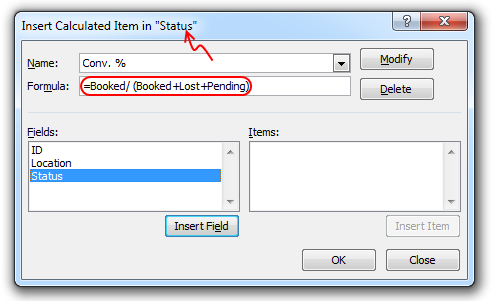
- Click ok.
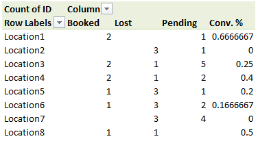
Now you should see another column in your pivot table with calculated item – Conversion %.
Formatting Conversion % in Percentage format
While we got what we wanted, it is not looking alright. We need to format the conversion % so that it looks alright. For this,
- Right click on any value in pivot table
 Go to value field settings
- Click on number format
- Select custom
- Type the custom formatting rule [>=1]0;[<1]0%;””
- This will automatically transform all numbers smaller than 1 (ie all conversion %s) to percentage format while keeping everything else normal.
- Done!
Resource: Learn more about custom number formatting
A video tutorial explaining this & more
Since calculated items can be somewhat tricky, I made a short video explaining how this works. In the video you can also see how to use Power Pivot measures to calculate conversion ratios easily. Watch it below (or on our youtube channel).
Download Example workbook
Click here to download example workbook. It has both regular and powerpivot based calculations. Go ahead and examine them. Enjoy.
Do you use Calculated items?
I find calculated items to be very tricky to work with. In most cases, I try to add extra calculations to original data table or use formulas instead. But this example is a good case where calculated item is perfect.
What about you? Do you use Calculated items? In what situations you use them? Please share your experiences and tips using comments.
Convert your self to a Pivot table pro…
If you are use Excel pivot tables & data analysis features, then you will find below resources very useful.


15 Responses
Great post. I still have trouble at times deciding whether I need a calculated ITEM or FIELD. This is very helpful.
Probably an obvious answer, but I’m missing it — why the custom number format for anything >= 1 as number. Why not leave it a percent, which would be 100%? Wouldn’t that be what we want it to show? The only time it would be 1 is when all were booked, so that would be 100%, right?
Thanks!
how is this different from calculate field.
I found this [>=1]0;[<1]0%;”” had to be changed to [>=1]0;[<1]0%;””
small difference but might be worthwhile to someone.
Chandoo, keep up the good work tks
Awesome! I should probably start using this tip in generating digital marketing reports! Pivot tables #FTW
Field is better option
Hi,
I would like how do you do the same with PowerPivot?
In PowerPivot, the option to insert “calculated item” is not available.
thanks,
Alyssa
Yes, I would like to know this too.
I have one query,
how to find out difference between two details & get the result of difference
Example
ABC ABC
BCD BCE
In the first in answer should be ABC
In the Second It should be BCE as its updated. kindly suggest.
How would you do a cumalitive sum calculated in a pivot table?
Nevermind, I figured it out.
Anybody,
What is the difference between Calculated Item and Calculated Field?
In the downloaded file there is “Grand total” for each row. But it sums up conversion ratios also, and it seems useless.
This Site Really Contain Good Info.
Hi there,
I’m trying to do a progress spreadsheet that will track monthly progress, by tying one worksheet (with pivot) to another that will also convert figures from the pivot into a chart on a separate worksheet. But what if there was nothing for a few months? What is the best command or formula to use to pick up that for some months, there is 0?
Please help. Thanks.
For the above example, if the location is divided into countries (adding another row label), does the calculated item work??
Thanks