
Its Friday, that means time for another Excel challenge for you.
This is based on yesterday’s employee vacation dashboard.
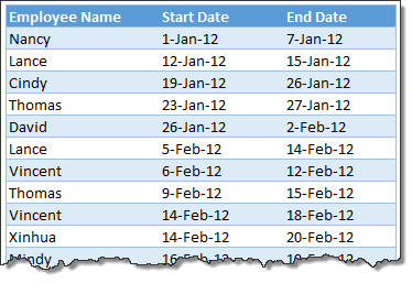
Calculate vacation days in a period:
 Your mission, if you choose to accept it,
Step 1: Download this workbook.
Step 2: Calculate number of vacations taken in a period. Specifically,
- How many vacations are taken between start & end dates, assuming complete vacation should be inside the start & end date period?
- How many vacations are taken such that at least one day of vacation is between start & end dates?
- How many people took vacations? (if same person took multiple vacations, then count it as 1)
You are free to,
- Use helper columns
- Any formula
- Play Mission Impossible music in background
- Drink no more than 2 cups of coffee
How to post your answers?
Simple, just post them in comments. Include explanation of your logic too if possible. Click here to post your answers.
Need some clues?
We have them. See these links:
GO!!!
Added later: Solution for this problem
here were quite a few interesting solutions in the comments.
Today, let me explain how to solve these problems using Excel formulas.
Watch below video:
Download solution workbook
Click here to download the solution work book & see the formulas.


67 Responses
Hi ,
I think this time , your challenges are quite simple ; I would like to add some more challenges :
How many of the vacations overlapped with each other ?
How many vacations did not overlap with each other ?
What is the maximum number of people who were on vacation at any point of time ?
What is the maximum period when at least one person was on vacation ?
What is the maximum / minimum period when no one was on vacation ?
Probably each of these can be taken up for a forensic post , assuming that each of them can be solved using formulae.
Please Provide the Answers
OK,
I’ve tackled 1) and 2) in similar ways, using COUNTIFS as follows:
1) =COUNTIFS(vacations[Start Date],”>=” & start,vacations[End Date],”<=” & end)
Counts number of vacations where Start Date is on or later than 01-Feb and End Date is earlier than or on 31-Mar – so entire vacation is within period.
2) =COUNTIFS(vacations[Start Date],”>=” & start,vacations[Start Date],”<=” & end) + COUNTIFS(vacations[Start Date],”<=” & start,vacations[End Date],”>=” & start)
Similar to 1st question, but looking for vacations where Start Date is later than 01-Feb and start date is earlier than 31-Mar – this captures all vacations that start in the period. Only vacations that are missing are those that start earlier than period and end once the period has started, which is captured by the
+ COUNTIFS(vacations[Start Date],”<=” & start,vacations[End Date],”>=” & start)
counting all records where start date is earlier than period start, and end date is later than period start.
3) There’s probably a nice array formula for this, which I’m going to try and work out. In the meantime, I added a new column, with the formula against the first row as:
=IF(AND([@[Start Date]]>=start,[@[End Date]]<=end,SUMIF($B$3:B3,[@[Employee Name]],$E$3:E3)=0),1,0)
So record a 1 if the vacation is fully within the period (start date is later than 01-Feb AND end date is earlier than 31-Mar) AND if the Employee concerned doesn’t already have a 1 against them.
I hadn’t used SUMIFS until I spotted it on Chandoo a few days ago – such a simple and powerful formula, and I took a guess that a COUNT version would also exist – I’m going to be using these a lot – thanks Chandoo!!
Interesting!
Hi ..
I tried to use your formulas which is really interesting but it doesn’t work with me 🙁
https://dl.dropbox.com/u/69797926/vacation-calculations_tadovn.xlsx
Dear,
I sent the answer for this.
I use helper column to calculate.
The formular i used is IF, COUNTIFS, SUM, SUMIFS.
Thanks,
Hi,
I have converted the Table as normal cells & also additional column (Col E).
Employee Name –
B4
Start Date –
C4
End Date –
D4
# of days –
E4
1. E4 to E123 – =SUMPRODUCT(–(ISNUMBER(MATCH(ROW(INDIRECT(C4&”:”&D4)),ROW(INDIRECT(start&”:”&end)),0))))
Q1 – =SUMPRODUCT(($C$4:$C$123>=start)*($D$4:$D$123<=end))
Q2 – =SUMPRODUCT(–($E$4:$E$123<>0))
Q3 -=SUM(IF(FREQUENCY(IF($B$4:$B$123<>””,IF($E$4:$E$123<>0,MATCH($E$4:$E$123,$E$4:$E$123,0))),ROW($E$4:$E$123)-ROW($E$4)+1),2))
@A. Ramanan
Hi..
Nice work but I wanna see Q3 form because it is not clear..
The answer for Q3 requires Ctrl + Shift + Enter
Some more challenges :
Who took the longest / shortest vacation , and for how many days ?
Who was on vacation for the maximum number of days ( this is different from the earlier question , since this includes more than 1 vacation by the same person ) ?
I need help
Problems running macros in Excel 2010 on Macintosh computers. How I can fix this?
Thx.
Below are the my solutions :
Q 1> =IF(C4>start,IF(D4<end,”YES”,”NO”),”NOO”) & Then =COUNTIF($I$4:$I$123,S3)
Q 2> =IF(AND(start<C4,C4<end),”YES”,IF(AND(start<D4,D4<end),”YES”,”NO”)) & then =COUNTIF($G$4:$G$123,S3)
Q3> Remove duplicates from Q 1
Hello everybody
Q1:
=SUMPRODUCT(–(vacations[Start Date]>=start),–(vacations[End Date]<=end))
Q2:
=SUMIFS(vacations[Column1],vacations[Start Date],”<=”&end,vacations[End Date],”>=”&start)
Column1= typed 1 in all cells parallel with other columns
Q3:
=IF(OR(C5<=start,D5>=end),IF(COUNTIF($B$4:B7,B7)=1,O4+1,O4),O4)
I get by this formula 13 people
Thank you
I am facing some kind of this problem.
My table is like this
“Start” column should have the same value as the “End” of Previous Row if the ID is same.
For example in the 1st row ID is 1 start and end is 0 and 20 respectively.
In the second row ID is 1. So the Start should be 20. But in table its 18. I need to find out the IDs that have this problem.
In third row ID is still 1 and “start” is equal to the End of Previous Row having ID 1. So its OK. Can any one give me idea? Thanks
ID
Start
End
1
0
20
1
18
40
1
40
230
2
0
250
2
250
1500
2
1500
1530
3
0
15
3
15
30
3
28
40
3
40
50
Could you upload excel file, pls?
Ans 1. COUNTIFS(vacations[Start Date],”>=”&start,vacations[End Date],”<=”&end)
Ans 2. Using a helper column with the number 1 in all rows, i used the formula: SUMIFS(vacations[Column1],vacations[Start Date],”<=”&end,vacations[End Date],”>=”&start)
Ans 3. I first removed the unique names and used the formula to find the dates using only unique names. Then i used the formula
Formula 1. COUNTIFS(vacations[Employee Name],O4,vacations[Start Date],”>=”&start,vacations[End Date],”<=”&end)
Formula 2. COUNTIFS(P4:P29,”>0″) to get 14 as the answer.
Thanks,
Mustafa
Hi the following are my answers:
Q1: =SUM((–((vacations[Start Date])>=start))*(–((vacations[End Date])<=end))) [CSE]
Q2: =SUM((–((vacations[Start Date])<=end))*(–((vacations[End Date])>=start))) [CSE]
Q3: This one was little tricky to do it in a single cell (without using helper column), so I copies all the names to a new column N, and removed duplicates (I found 26 unique names in this case) and in the next column I applied the following formula and dragged it down to the last row:
=IF(SUM(–(N4=vacations[Employee Name])*(–((vacations[Start Date])>=start))*(–((vacations[End Date])<=end)))>0,1,0) [CSE]
And, took a sum of all the velues which was equal to 14.
*CSE = Control+Shift+Enter
Thanks,
Raj Kumar Kothari
So the first two aren’t that hard but the third one was quite a pain to do in one cell. Since most people have already answered the first 2, I won’t bother answering those. But I will post an answer to the third one:
Enter this as an array formula:
=SUMPRODUCT(IFERROR(1/COUNTIFS(vacations[Employee Name],vacations[Employee Name],vacations[Start Date],”>” & start,vacations[End Date],”<” & end),0),–(vacations[Start Date]>start),–(vacations[End Date]<end))
The inspiration for this formula comes from a formula chandoo posted a while back on how to count the number of unique items in a list.
Thanks for the great challenge Chandoo!
Hi Mitch,
I copy pastes this formula but didn’t work.
–(vacations[Start Date]>start),–(vacations[End Date]<end) part of the formula yields an error,
Thanks,
Raj
The “-” should be doubled as in below (I copy/pasted it from excel before but it seems to have changed to single “-” by itself. I’m using excel 2007 (don’t know if that could cause the error)
=SUMPRODUCT(IFERROR(1/COUNTIFS(vacations[Employee Name],vacations[Employee Name],vacations[Start Date],”>” & start,vacations[End Date],”<” & end),0),–(vacations[Start Date]>start),–(vacations[End Date]<end))
Turns out it’s not my excel copying but the website that, for some reason, is autocorrecting it to not double the “-“.
You should have two “-” whenever you see them. Let me know if that works.
Hey Mitch, I tried using the double negative, but didn’t work.
Thanks, Raj
Try this. It has the spreadsheet.
http://www.excelforum.com/excel-formulas-and-functions/894788-unique-count-with-criteria.html?p=3100520#post3100520
Hi Mitch, Thanks for your efforts for sharing the link. I really appreciate your help. And yes, this your formula is working fine. Great trick.
Thanks , Raj
Hi Mitch,
Thanks for the solution. A question why we have two dash in front “–”
in the formula.
=SUMPRODUCT(–(vacations[Start Date]>start),–(vacations[End Date]<end))
Thanks
http://www.k2e.com/tech-update/tips/143-using-two-minus-signs-in-excel
to understand usage of double minus signs
Hi,
I have tried the below formule for the 3 questions.
1. How many vacations are taken in this period?
A: =SUMPRODUCT((vacations[Start Date]>=start)*(vacations[End Date]<=end))
2. How many vacations are taken in this period?
A: =SUMPRODUCT((vacations[Start Date]<end)*(vacations[End Date]>start))
3. How many distinct people took vacation in this period?
A: For this, i got some error when written in single cell. So i have taken one helper column. (Column E)
Filled the column E with ‘=IF(([Start Date]>=start)*([End Date]<=end),[Employee Name],”0″)’
Used the below formula to get the answer for the question.
=SUMPRODUCT(1/COUNTIF(vacations[Column1],vacations[Column1]))-1
Q-1 Actule Result will be 25 from 1st Jan.12 to 31st Mar.12 with below formula
=SUMPRODUCT(–(C4:C123>=start)*(D4:D123<=end))
@-2 & Q-3 Pls clear what result u want
Smarty
How can i join this group to get & give the Solutions
Smarty
@Smarty
Start here: http://chandoo.org/wp/welcome/
1. =COUNTIFS(vacations[Start Date],”>=”&start,vacations[End Date],”<=”&end)
2. =COUNTIFS(vacations[Start Date],”<=”&end,vacations[End Date],”>=”&start)
3. This isnt working, what am I missing? First of all, its giving me an extra ;0 in the 3rd array, and secondly, my formula isn’t correct, in the sense that the match range should correspond correctly.
=SUMPRODUCT(–(vacations[Start Date]>start),–(vacations[End Date]<end),IF(FREQUENCY(MATCH(vacations[Employee Name],vacations[Employee Name],0),MATCH(vacations[Employee Name],vacations[Employee Name],0))>0,1,0))
I guess an array would work..
Q3:
Column C in ascending order.
1) Column C even year:
M16: {=CORRESP(MÊS(start);MÊS($C$4:$C$123);0)+3}
M17: {=CORRESP(MÊS(end);MÊS($C$4:$C$123);1)+3}
M18: {=SOMA(1/CONT.SES(INDIRETO(“B” & M16 & “:B” & M17);INDIRETO(“B” & M16 & “:B” & M17)))}
2) Column C different years:
N16: {=CORRESP(DATA(ANO(start);MÊS(start);1);DATA(ANO($C$4:$C$123);MÊS($C$4:$C$123);1);0)+3}
N17: {=CORRESP(DATA(ANO(end);MÊS(end);1);DATA(ANO($C$4:$C$123);MÊS($C$4:$C$123);1);1)+3}
N18: {=SOMA(1/CONT.SES(INDIRETO(“B” & N16 & “:B” & N17);INDIRETO(“B” & N16 & “:B” & N17)))}
Question:
Suppose we have this 2 dates into the excel vacations file:
David: Start day: 25/01/2013 & End Day: 4/02/2013.
In this case David enjoyed 7 job days of his vacations. But also in my report i need to track how many vacations belongs to each month.
In this case the answer is 5 days for January and 2 days for February. But I cant figure out how to get this with any formula.
Thx for the help..
ERROR IN THE SOLUTION XLS
Well.. i noticed this for the question2 : how many vacations are taken in this period. With the current solution, any vacation starting before ‘start’ and ending after ‘end’ is calculated twice. An alternative approach to fix this is to subtract vacations starting after the period and vacations ending before the period from the total number of vacations. Here is the formula i used :
=COUNTA(vacations[Employee Name])-COUNTIF(vacations[End Date],”<“&start)-COUNTIF(vacations[Start Date],”>”&end)
Q1:
=CONT.SES(C4:C123;”>=” & start;D4:D123;”<=” & end)
Q2:
=CONT.SES(C4:C123;”>=” & start;C4:C123;”<=” & end) + CONT.SES(C4:C123;”<” & start;D4:D123;”>=” & start;D4:D123;”<=” & end)
Dear Friends,
i need someones help to over come the issue i am facing that is i need to remove first orlast letters from the content in a cell
Ex.
HEPLANDCCRDDSUA
last 2 digits, UA needs to be removed
HOw can i do this as i need to do this for more than thousand
Thank you,
Naveen
@Naveen
If it is always 2 characters
=Left(A1,Len(A1)-2)
Otherwise what are the rules for determining how many characters it is you want to keep
@Navin:
You can use the following formula and drag it down till the desired amount of cells: (Please change the referencing according to your data)
=MID(A1,1,LEN(A1)-2)
Thanks, Raj
hi Chandoo. i spotted a discrepancy in Q2’s answer. if you change C4’s date to be before the Start Date & D4 to be after the End Date, the formula double counts that cell.
hence, maybe:
=SUMPRODUCT((vacations[Start Date]<start)*(vacations[End Date]>=start)+(vacations[Start Date]>=start)*(vacations[Start Date]<=end)*(vacations[End Date]>end))
or:
=COUNTIFS(vacations[Start Date],”<“&start,vacations[End Date],”>=”&start)+COUNTIFS(vacations[Start Date],”>=”&start,vacations[Start Date],”<=”&end,vacations[End Date],”>”&end)
i love your dashboards by the way
Hi Benishiryo, Even I am getting incorrect answer with both the solutions provided by you. Please try below:
=J8+COUNTIFS(vacations[Start Date],”greater than”&start,vacations[End Date],”greater than equal to”&start)+COUNTIFS(vacations[Start Date],”less than equal to”&end,vacations[End Date],”greater than”&end)
=COUNTIFS(vacations[Start Date],”>=”&start,vacations[Start Date],”=”&start,vacations[End Date],”=”&start,vacations[End Date],”<="&end)
My answer for q2
Reg the video.. I am getting incorrect answers for the second question. if there are vacations that are on the exact start date and end date as specified as start and end.
Even if one day of the vacation is between start and end dates, you should count it
I am getting correct answer with following:
=J8+COUNTIFS(vacations[Start Date],”=”&start)+COUNTIFS(vacations[Start Date],””&end)
In the video it was mentioned as following, which seems to be incorrect.
=J8+COUNTIFS(vacations[Start Date],”=”&start)+COUNTIFS(vacations[Start Date],”=”&end)
Please correct me if I am wrong.
probably not the most sussinct ones, especially for the Q3:
Q1==SUMPRODUCT((vacations[Start Date]>=start)*(vacations[End Date]<=end))
Q2=SUMPRODUCT((IF(((start<=vacations[Start Date])*(vacations[Start Date]<=end))+(start<=vacations[End Date])*(vacations[End Date]0,1,0))) CSE
Q3=SUMPRODUCT(1/(COUNTIF(INDEX(vacations[Employee Name],MATCH(1,(vacations[Start Date]>=start)*(vacations[End Date]=start)*(vacations[End Date]=start)*(vacations[End Date]=start)*(vacations[End Date]<=end),0)),G8-1,0)))) CSE
some rearrangements for Q3 to avoid constant referrence (1) in the MATCH function. it may be useful in case of the same task with Q2 conditions
Q3=SUMPRODUCT(1/(COUNTIF(INDEX(vacations[Employee Name],ROWS(C4:INDEX(vacations[Start Date],MATCH(TRUE,vacations[Start Date]>=start,0))-ROW(C4)+1)):OFFSET(INDEX(vacations[Employee Name],ROWS(C4:INDEX(vacations[Start Date],MATCH(TRUE,vacations[Start Date]>=start,0))-ROW(C4)+1)),G8-1,0),INDEX(vacations[Employee Name],ROWS(C4:INDEX(vacations[Start Date],MATCH(TRUE,vacations[Start Date]>=start,0))-ROW(C4)+1)):OFFSET(INDEX(vacations[Employee Name],ROWS(C4:INDEX(vacations[Start Date],MATCH(TRUE,vacations[Start Date]>=start,0))-ROW(C4)+1)),G8-1,0)))) CSE
For the first two parts I had a slightly different answer, which seemed a little simplier than the given answers (they are both array formulas, and so require control-shift-enter):
Part 1:
=SUM(IF(vacations[Start Date]>=start,IF(vacations[End Date]=start,IF(vacations[Start Date]<=end,1,0),0))
What is posted above is not my formula. Somehow it was muddled in the posting process. I will try again:
Part1:
=SUM(IF(vacations[Start Date]>=start,IF(vacations[End Date]=start,IF(vacations[Start Date]<=end,1,0),0))
Both array formulas, use with control-shift-enter.
Muddled again. I give up.
hmmm…I got two out of three, and when I check the third mine result coincides with the data
How many vacations are taken in this period?
=COUNTIFS(vacations[Start Date],”>=”&start,vacations[End Date],”=”&start,vacations[End Date],”<="&end)
+COUNTIFS(vacations[Start Date],"<="&start,vacations[End Date],"=”&start)
+COUNTIFS(vacations[Start Date],”>=”&start,vacations[Start Date],”=”&end)
How many distinct people took vacation in this period?
For this I inserted a column in the table, starting in the first row, then copying this down
=IF(AND(OR(AND([@[Start Date]]>=start,[@[End Date]]<=end),AND([@[Start Date]]<=start,[@[End Date]]=start),AND([@[Start Date]]>=start,[@[Start Date]]=end)),COUNTIFS(C$3:C3,”=1″,B$3:B3,”=” &[@[Employee Name]])<1),1,0)
Then in H19 (the answer cell) =SUM(vacations[Column1])
That gave me 15…even hand-counted and sorted for dupes…maybe corrupted my file with a wrong date?
Name Start Date End Date
David 1 26-Jan-12 2-Feb-12
Lance 1 5-Feb-12 14-Feb-12
Vincent 1 6-Feb-12 12-Feb-12
Thomas 1 9-Feb-12 15-Feb-12
Xinhua 1 14-Feb-12 20-Feb-12
Mindy 1 16-Feb-12 19-Feb-12
Cindy 1 18-Feb-12 21-Feb-12
Albert 1 19-Feb-12 22-Feb-12
Jackie 1 24-Feb-12 4-Mar-12
Zack 1 29-Feb-12 3-Mar-12
Ganesh 1 1-Mar-12 7-Mar-12
Queen 1 3-Mar-12 5-Mar-12
Barry 1 7-Mar-12 9-Mar-12
Wendy 1 13-Mar-12 17-Mar-12
Steve 1 17-Mar-12 21-Mar-12
Not a fan of array formulas but the task was fairly small so no impact.
={SUM(1/COUNTIF(INDIRECT(ADDRESS(MATCH(start,vacations[Start Date])+4,2,1,1)&”:”&ADDRESS(MATCH(end,vacations[End Date])+3,2,1,1)),INDIRECT(ADDRESS(MATCH(start,vacations[Start Date])+4,2,1,1)&”:”&ADDRESS(MATCH(end,vacations[End Date])+3,2,1,1))))}
1. Answer=COUNTIFS(vacations[Start Date],”>=”&start,vacations[End Date],”<="&end)
2. Answer=COUNTIFS(vacations[Start Date],"=”&start)
3. I used 2 helper columns – one to test the vacation dates and enter the name of employee and the other to count the employee if it was unique and ignore blank space and duplicate employee names.
column1=IF(AND([@[Start Date]]>=start,[@[End Date]]<=end),[@[Employee Name]],"")
column2 =IF([@Column1]="",0,IF(COUNTIF($E$1:E3,[@Column1])=0,1,0))
Answer=SUM(vacations[Column2])
I am not sure if this has already been addressed but here goes:
I am tracking vacation taken by employees. I want to be able to tell if there is a vacation conflict between two people from the same departement.
Also, since they are not required to take all their days at once, I have set up 4 vacation periods per person.
John — Acct 7/1 – 7/20
Bob — Sales 7/5 – 7/25
Evan — Acct 7/5 – 7/25
I would like for John and Bob’s names and vacation days get highlighted to show conflict.
Thank you in advance
Took a long time to figure out 3. These are the formulas I have used.
1. =COUNTIFS(vacations[Start Date],”>=”&start,vacations[End Date],”<="&end)
2. =COUNTA(vacations[Employee Name])-COUNTIFS(vacations[End Date],"”&end)
3. Used a helper column (column E) which populates with a “N” if the start and end dates of vacations do not fall within the specified date range. It populates the first within-range instance of a recurring person with a “Y”. Any subsequent vacation occurences by the same person are populated with a “N”.
Formula in helper:
=IF(AND(COUNTIFS($B$3:B3,[@[Employee Name]],$E$3:E3,”=”&”Y”)=0,[@[Start Date]]>=start,[@[End Date]]<=end),"Y","N")
Don’t you think, the below formula works for the question no. 2
=COUNTIFS(vacations[End Date],”>=”&start,vacations[Start Date],”<="&end)
Counting Unique Values is a very, very useful skill. I use a countif with a fixed and non-fixed array then use the “1” values to determine which are “new unique values.”
=IF([@[Vacation Name]]=””,””,(COUNTIF($K$4:K4,K4)))
the sample output is:
Vacation Name Unique Count?
Lance 1
Vincent 1
Thomas 1
Vincent 2
Xinhua 1
Mindy 1
Cindy 1
Albert 1
Jackie 1
Zack 1
Ganesh 1
Queen 1
Barry 1
Queen 2
Jackie 2
Xinhua 2
Wendy 1
Albert 2
Thomas 2
Steve 1
Greetings.
For Q1 I use Column M to set this formula
=IF(AND(C4>=$K$3,D4=$K$3,C4=$K$3,D4<=$K$4)),1,0)
Then I just autoSum the Column
For Q3 I use the results from Column M and I just extracted the name values with this formula =IF(M4=0,"",B4) in Column O. With just the names of the people who took a vacation during that period, I just copy, special paste, and applied Data tools-Remove duplicates. This allowed me to count the people on vacation during that period.
Thanks. Good Challenge.
My way just showed you all that there are at least 100 ways to evaluate something in Excel, you just need the proper logic.
Q1: there are several ways to display the response. all have been posted before:
A1-1=COUNTIFS(vacations[Start Date],”>=”&start,vacations[End Date],”=start)*(vacations[End Date]=start),–(vacations[End Date]<=end))
Q2: same answer by simply changing start and end around.
A2-1 =COUNTIFS(vacations[Start Date],"=”&start)
A2-2 and A2-3 follow above
Q3: I really like Mitch’s solution. I came to the same after a few iterations.
A3 ={SUMPRODUCT(IFERROR(1/COUNTIFS(vacations[Employee Name],vacations[Employee Name],vacations[Start Date],”>=”&start,vacations[End Date],”=start)*(vacations[End Date]<=end))}
theory: if an event is counted more than once in a sample, then SUM(1/COUNT(events)) = 1. For example, an event counted 3 times will post as 1/3; 1/3; 1/3 with SUM(1/3,1/3,1/3) = 1
Note on SUMPRODUCT: One can replace the "*" multiplier by comma "," and using the double negative "–".
The "–" replaces TRUE and FALSE by 1 and 0. Use "*" to "multiply" arrays when performing SUMPRODUCT on TRUE and FALSE; use "," array separator when performing SUMPRODUCT on 1s and 0s.
Alternative Solution:
1. =SUMPRODUCT(–($C:$C>start),–($D:$D<end))
2. = SUMPRODUCT(–($C:$Cstart))
3. I hate helper columns. I have yet to figure it out how.
Hi there, I think you have an error on the “How Many vacations are taken in this period.
If the holiday start date is pre the range and the holiday end date is post the range the formula calculates this as 2 holidays. If you do have a correct formula for this calculation I would be grateful as I have exactly the same issue. Many Thanks
I did it in a simple way and it worked.
Note: My excel is in portuguese pt-br
Q1: =CONT.SES(C:C;”>=”&start;D:D;”<="&end)
Q2: =CONT.SES(C:C;"=”&start)
Q3: I’ve just copied the answer. I confess I would’ve never thought about the solution given.
Hello
Could someone tell me how to solve Q2 in below workbook
https://chandoo.org/wp/calculate-vacation-days/
I am a beginner so, I assume my solution is simpler and understandable by all. I used helper columns and some basic formulas like: counta, if(), unique() ect…
Here is the link:
https://docs.google.com/spreadsheets/d/1gTfTYeLI5b6IBgApZRS0seB4A6qCvFdg/edit?usp=sharing&ouid=104412430299715464739&rtpof=true&sd=true
I think I did well for the most part. Last question was a bit of a hassle but it works and it’s adaptable.
Q1: =COUNTIFS(vacations[Start Date],”>=1-Feb-12″,vacations[End Date],”=1-Feb-12″,vacations[Start Date],”=start)*(vacations[End Date]<=end)
Column F's Formula: =IF(E9=0," ",vacations[@[Employee Name]])
Column G's Formula:=UNIQUE(F9:F28)
Column H's Formula:=COUNTIF(G9#,"*")
Make the 1's and 0's array, use the if to print each name with a 1, use the unique function to get each unique name, and countif with wildcard to count the number of unique names
Nice solution, but it will make some errors!!!
Try start date in the table vacations end date.
I’ve tried with Thomas: strart date 23-JAN end date 27-JAN, just change end date to 27-MAY so the answers are:
q1 – without changes – however it shoud be so, becauses vacation didn’t start in required time frame.
q2 – ansewr is 24 – and that is wrong.
q3 – without changes – it’s correct, but should be aware, key word here is “took vacation”, and if you are interested in how many people were in vacation it will not give you correct answer!
q1:=COUNTIFS(vacations[Start Date],”>=01-02-2012″,vacations[End Date],”=01-02-2012″,vacations[Start Date],”
=IF(AND(B4>=DATE(2012,2,1),B4 =COUNTIFS($D$4:D4,D4,$D$4:D4,”NA”)
q3:=COUNTIF(vacations[dummy 2],1)
Q1: =COUNTIFS(vacations[Start Date], “>=”&start, vacations[End Date], “=”&start, vacations[End Date], “=start)*(vacations[End Date]<=end))))
Q1: =COUNTA(FILTER(B:B,(C:C>$K$3)*(D:D=” & start,C:C,”<=" & end)+COUNTIFS(D:D,"=” & start)-COUNTIFS(C:C,”>=” & start,D:D,”$K$3)*(D:D<$K$4))))