Moosa, one of our readers emailed this interesting question:
I have huge list of customers (around 1500).
Table includes following information
Customer # , Customer Name, Sales 2002, sales 2003, … sales 2012My requirements are
1. list of customer who did not have sales during all these years
2. List of customer who have not business from 2002
3. List of customer who have not business from 2003
…
10.List of customer who have not business from 2012
So how do we identify these customers?
Of course, we can write a very long and complex formula to get the list. I think we are better off using that energy to reach out to these customers and improve the sales. So lets figure out an easy solution.
Enter Pivot Tables
Assuming our data looks like this:
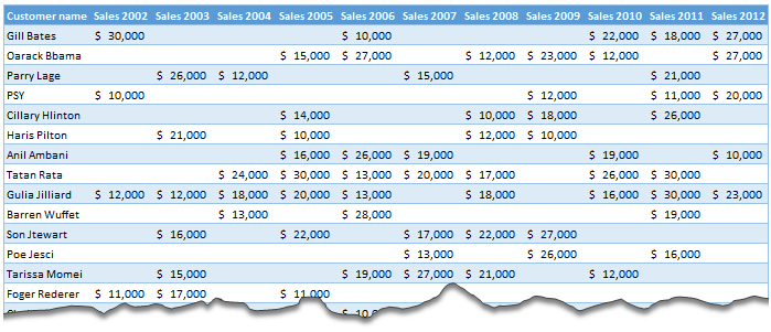
1. Select any cell and insert a pivot table
2. Set up pivot table like this:
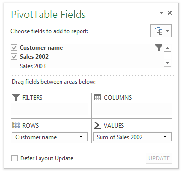
3. Add Value filter show only customers with sales
Click on row label > value filter and set up criteria like this:

[More: using value filters with pivot tables]
4. Our report for non performing customers in 2002 is ready!
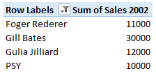
Hmm.. this good, but tedious
You are right. Although this approach gives answer for a particular year, when we want results for another year, we need to repeat all steps again. Not cool man, not cool.
So what next?
Part of the problem is due to how our data is structured. If we had 3 column structure like below,
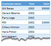
we could set up a report filter on year and see which customers did not have any sales for any given year.
Alas, lets assume Moosa is stuck with this data.
Enter a helper column
We could improve our original solution so that user can select any year (or all) and see which customers did not fetch any sales by using a simple helper column.
- Just go to the original data set and add an extra column at the end.
- Call this selected year
- Now, go to an empty cell somewhere else in the worksheet and name it asselYear
- This is where we will keep the year for which we want the results (can be 2002, 2003…2012 or all)
- Lets assume our data is in range C4:M4 (C4 has 2002, D4 has 2003 … M4 has 2012)
- Now, we want to fetch only the selYear’s data in to this helper column. So if 2002 is selected, we want data in C4, for 2003 data in D4… and for all we want sum of all numbers in C4:M4.
- Looks like we can use some INDEX magic here.
- In the helper column write
=IF(selYear="all",sum(C4:M4),INDEX(C4:M4,selYear-2001)) - Go ahead and examine that formula. I am not going to explain 😛
Now, our helper column fetches any one years data or sum of all years data, based on what users want. Awesome!
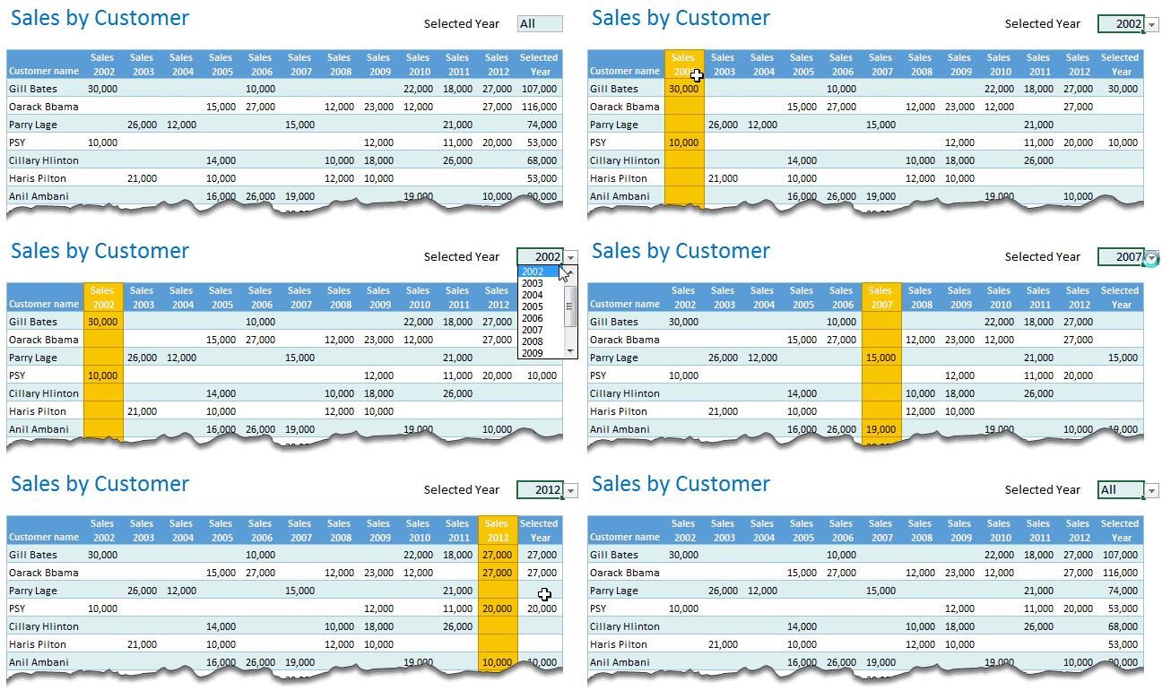
Lets go back to the pivot
Armed with our helper column, lets re-create the pivot table. But this time, instead of dropping any one year, we will drop selected year column in to “Values” area. This way, our pivot report shows customer names for selected year.
Lets add a combo-box form control so that we can select the year interactively.
But there is one problem!
Our pivot report does not refresh whenever we select another year.
Of course, we can easily fix this with a one line macro & some duct tape.
Right click on the combo box and choose “Assign macro”
Name the macro as refresh Pivot and write below code [more on the macro here]
Sub refreshPivot()
ActiveWorkbook.RefreshAll
End Sub
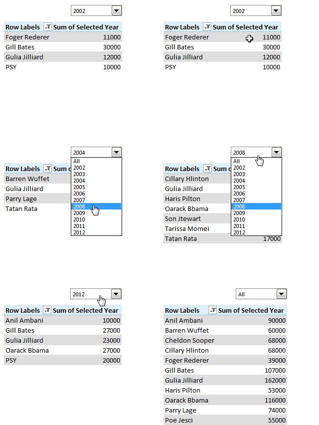
And we are done! We can interactively see which customers did not fetch us any sales for any given year. See this demo:
Download Example workbook
Click here to download example workbook & see this in action. Explore the macro & pivot table settings to understand how this works.
Using Pivot tables vs. Formulas for cases like this
I think this is a perfect example when Pivot table based solution is simpler compared to formula based one. Not only is it simple to set up, but it is very usable & modifiable. Often we complicate a problem by trying to figure out the perfect formula for it. I think an intelligent Excel user needs to mix various options – pivot tables, vba, formulas, tables etc. to get the solution in few simple steps.
This way, we can spend rest of our time finding out why Foger Rederer never bought anything from us after 2005.
What do you think? Do you use pivot tables often? How would you have solved Moosa’s problem? Please share using comments.
Learn Pivot Tables & Become a data rock-star
If you are new to pivot tables or have not used them to their full potential, now is the time to dip your toes. Check out below resources:
- Introduction to Excel Pivot Tables
- My top 5 tips for Pivot Tables
- How to group data in pivot tables
- Using slicers to filter pivot tables – new feature in Excel 2010
- Using report filters
- Visit our extensive pivot table section
Consider joining in our Excel School program: If you want to learn how to combine formulas, pivots, conditional formatting, charts & various other features of Excel to do awesome stuff, then please consider joining my Excel School program. It is a completely online course designed to make you awesome in Excel and Dashboards. To know more and join us, please click here.


One Response to “How to create SVG DAX Measures in Power BI (Easy, step-by-step Tutorial with Sample File)”
My intention in this leave tracker, is to see other months instead of last 3 months of the year