Today I want to introduce a new excel feature to you, called as Picture link.
Well, picture links are not really new, they are called as camera snapshots in earlier versions. They provide a live snapshot of a range of cells to you in an image. So that you can move the image, resize it, position it wherever you want and when the source cells change, the picture gets updated, immediately.
What is the use of Picture Links or Camera Snapshots?
At the outset picture links may seem like a useless feature. But they are pretty powerful. Here are few sample uses for picture links:
- In dashboards & reports: Usually in dashboards, we need to combine charts, tables of data, conditional formatting etc., all in one sheet. When the size of these are not uniform, aligning them on output sheet could be a huge pain. This is when you can use picture links. First create the individual portions of dashboard in separate worksheets. Then, embed picture links to these portions in final dashboard. Re-size them and align as you see fit.
See this in action: Project management dashboard in excel
. - In micro-charts & sparklines: While Excel 2010 has native support for sparklines and other micro-charts, if you want to create a micro-chart in earlier versions of excel you have to use trickery. This is where picture links can help. You can make a regular chart and take a picture link of that. Then resize the picture so that it fits in to a small area.
See this in action: Micro-charts using camera tool.
- In Dynamic Charts: Since picture links are nothing but images with a formula assigned to them, you can easily construct dynamic charts & dynamic dashboards using these.
See this in action: Dynamic chart using camera tool, Dynamic dashboard using camera tool
- In shared workbooks: When you share a workbook with a colleague or boss, a common worry is what if they change formulas or edit something. This is where picture links can be of great use. You can embed a picture link of actual data so that no one can edit it.
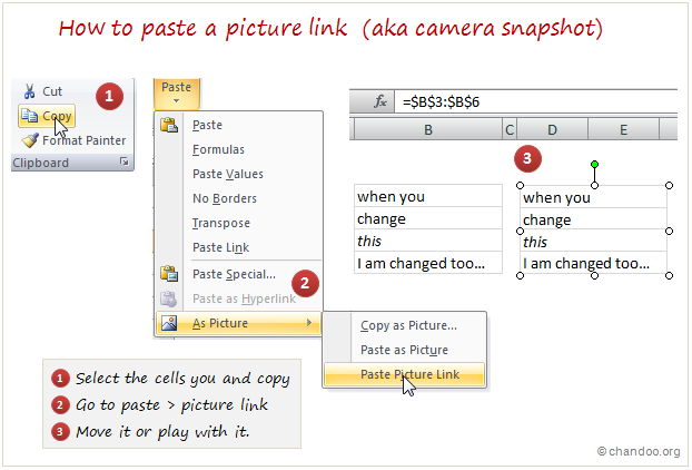
How to insert a picture link in Excel – 3 step tutorial:
To insert a picture link to your data, just follow these 3 steps:
- Select the cells. Press CTRL+C
- Go to a target cell. From home ribbon select Paste > As picture > Picture link option (see image below)
- That is all. Your picture link is live. Move it or play with it by changing source cells.

Do you use Picture Link / Camera Snapshot ?
I have been a fan of picture links / camera snapshots ever since I learned about them. I have used them in various dashboards, reports, workbooks to wow my clients, bosses and colleagues. However, one problem with picture links / camera snapshots is that, they do not print well. So I avoid using them for workbooks that get printed alot.
What about you? Do you use picture links often? Share your experience, tips and ideas using comments.
Read more quick tips to become awesome in excel, in less than a minute.
PS: Donut to Hui for telling me about Picture links feature.


35 Responses to “Quick and easy Gantt chart using Excel [templates]”
"Please share your experiences and ideas using comments"
For those willing to go VBA, XL can do far more w/Gantt Charts. Compare to PapaGantt. https://sites.google.com/site/beyondexcel/project-updates/papagantt-thebigdaddyofxlganttcharts
While making PapaGantt was neither quick nor easy, using PapaGantt is both, not just for displaying Gantts, but for scheduling tasks as well.
is it possible to get a xls(m) file ?
instead of a zip-file with .xml-files ?
i cannot open it with excel :/
Regards
Stef@n
@Stef@n
Try saving the file and then open from Excel as opposed to opening directly from the post
Also try this link: http://img.chandoo.org/pm/quick-gantt-chart-template.xlsx
Thanks very much for this workbook idea.
To slightly up-scale functionality I added:
1. conditional format for when the cell value =2 to be red which could be used for critical path or other activity highlighting needs (milestones perhaps)
2. conditional format for when the cell value =c to be green which could be used for showing activity progress
3. conditional format for the same range where formula =DATE(YEAR(D$5),MONTH(D$5),DAY(D$5))=TODAY() and set custom to ;;; and cell fill colour to a light blue. This will highlight today down the whole table to allow quick assessment of activity progress to plan. Anything not green upto where the date indicator is shows activity is behind the plan. Opposite for tasks ahead of the plan.
(There is probably a better way to get the same result but this works for now. If there is please post for us to share.)
Hope this made enough sense.
Also, thanks Craig for the link. I'll have a better look soon.
Regards,
Darren
Hey Chandoo,
I actually made one of these for a friend of mine but added an extra level of automation.
Rather than putting in 1 on all the dates the activity occurs, I added a column for start and end date of each project. Then I used formula along the lines of :
=IF(AND(DateAtTop >= Start Date, DateAtTop <= End Date),1,"")
Then used the same conditional formatting where 1 was coloured.
I thought this was a nice touch, especially if a project lasts for many days.
Let me know what you think 😉
Lucas
P.S. First time I've posted here, love your work btw!
Hi Lucas... welcome to the comments and thanks for your first of many comments.
I like the idea. In fact, it was one of the first Excel tricks I ever learned (to use conditional formatting to automate things like this). See this (written almost 6 years ago)
http://chandoo.org/wp/2008/03/13/want-to-be-an-excel-conditional-formatting-rock-star-read-this/
and scroll-down to the tip on gantt charts. 🙂
I liked this approach and tried adding it into the Conditional format via Formula = statement. It workd fine with just the AND statement but then I realised you need the "1"'s to calcluate the duration.
I then put the whole IF statemnt in but it hasnt worked. Any thoughts?
Ta
Hi Lucas and Darren,
I tried the conditional formatting but I really don't succeed in getting the solution. Do you have a template of this?
Thanks in advance
Br
[…] http://chandoo.org/wp/2014/02/18/quick-gantt-chart-excel-template/?utm_source=feedburner&utm_med… […]
[…] via Quick and easy Gantt chart using Excel [templates]. […]
Excellent, thanks for this tip and expample.
I had a monthly reporting template very similar to this, but was done in excel which needed more manual inputs.
I used your exmaple and updated my monthly group reporting plan.
I further devided the day into 4 quarters to make it easy for us to followup on different tasks.
Now, I just have to update the start date, and everything gets udpated by itself in fraction of a second.
Thanks once again. love your daily udpates.
Wow.. glad to hear that.
Hi Prahlad,
Can you share ur template even i am looking for similar kind of template .where i want day duration ,split in hrs and each task effort represented in hr spent by each resource .
Thanks
savi
Hi Chandoo,
Can you guide on preparing an indian version of the captioned sheet. We have saturdays working :-(, and only one day weekly off on sunday.
Regards-Prajay
Hi Chandoo,very useful post.i need gantt chart for inventory module.
[…] Quick and easy Gantt chart using Excel […]
Hi.
Really usefull post. I would like to know if i can also include weekends.
Thank you
Hi Chandoo, thank you for the great job, I was wondering if you can customize this sheet for Inventory planning purposes?!
thank you indeed
This was so helpful. ive been through about 10 different tutorial type things and this has to be the best so far, helped me out a great deal. and now my boss is happy i can make gantt charts!
thanks
This's a great post, thanks for sharing
Hi Chandoo,
Thanks for the excel tutorial. I wanted to make a simple modification, however it will cause issues with the duration part. I created another rule/cell marked 2. For my project I want to show a projected timeline and then an actual timeline. The issue is that the duration is being logged for when I enter 2, which I want to be projected and not actual. Will you please assist in letting me know how I can create a duration for both project and actual on the same line?
Thank you,
Steven
Showing vertical line between every week is very useful for me, I used to do it manually. Thanks so much!!
But how about, my gantt chart included Saturday & Sunday, and I want to show the vertical line after Sunday, could any expert teach me how to fix it. Thanks again.
This was so helpful - thank you! I had a bit of trouble with the end of the week conditional formatting over-writing the filled cells but switching the order of the rules sorted it out. Needed to put together a gantt chart quickly for an important bid at short notice and this was just the job - thanks for taking the time to post it. Much appreciated.
This is the first time I'm reading a tutorial that actually makes sense 🙂 This is absolutely great, with only one minor issue I can't seem to figure out on my own. How do I include weekends in (or instead of) the Workday formula? Thank you!
[…] This template I made myself but I inspired from Chandoo.org. […]
Hi,
Sometimes I must work at weekends - it is possible to modify the dates so that you can include Sat + Sun as well?
Thanks,
H
Nice gantt chart template chandoo, simple but useful
Thank you so much for this excellent guide! I have adapted this to show scheduled activities at multiple project sites weekly over the course of the year, including active and proposed work. With just a tiny bit of tweaking to your tutorial, I was able to create a chart that suited my needs perfectly!
Thank you very much for idea sharing .very innovative workday formula is showing 5 days but i want 6 days , is there any other option plz reply..
i got it friends..
=WORKDAY.INTL(F4,1,11)
hhhhhh
@Somnath
I also like the structure using =WORKDAY.INTL(F4,1,"0000001")
where each day is a 0 or 1
Hi thanks a lot for the tuto!! It helped me a lot!!
But can you tell me how can I add a vertical line representing today on it?
@Cynthia
Open the template
Select D7:DS26
Goto Conditional formatting
New Rule
Use a Formula
=D$5=today()
then set the format as a Red Right Hand Border only
Apply
Do not select stop here for the rule
Hi Chandoo,
I purchased your Project Management templates a month ago and have not had the chance to thank you for the great templates. Thank you!!!!! It has saved me a lot of time creating and re creating templates. Unfortunately, I had to do a lot of customization but it's not that bad. I am now in the process of customizing my GANTT which my boss thinks is too granular. He doesn't want to see a weekly grant. Only the months should be showing. I have researched and researched but to no avail. Do you have any examples I can look at?
Hi Chandoo,
thanks so much for all your tips on Gantt Table.
I'm actually building one at the moment and want to use the conditional formatting. However, I always get into trouble with that when I have to add new lines. I don't know the final size of my table yet and I eventually also want other people to be able to work with it.
Conditional formatting tends to "split up" into various "applies to" ranges when you insert a new row or copy and past values from somewhere.
I'm sure you've come across this issue already... So far I couldn't find a feasible solution to this. I was wondering if you had an idea / suggestion for me?
Thanks so much!!!
Nadine