Data Validation using an Unsorted column with Duplicate Entries as a Source List

Share

Facebook
Twitter
LinkedIn

This is a guest post by Hui, our in-house excel ninja.
Data Validation using an Unsorted column with Duplicate Entries as a Source List

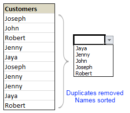
Here is a typical scenario: We want to allow only one of the pre-defined customer names in our spreadsheet. We have listed down all the customers in column B and want excel to check against this list and validate the data. But there are 3 problems. (1) Our list is not sorted alphabetically (2) It contains duplicates and (3) The list comes from external source, so we can not remove duplicates and sort the list every time.

Now how can we set up a simple data validation list that would not repeat customer names and shows them in sorted order like this:
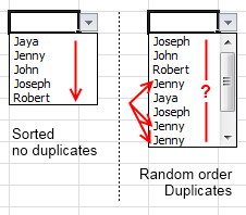
sorted-vs-jumbled-data-validation-lists

Here is the solution:

We need to remove duplicate entries and sort our data before it is fed to data validation list source. For this, there is a perfect tool right inside excel.

The rapid sorting cat.

Well, I am kidding. We use pivot tables. Pivot tables can sort the data as well as remove any duplicates. We can construct list of unique and sorted customers as column headers.

Just follow these simple steps:

  1. Select the source customer list and make a new pivot table. Insert the pivot table in the same sheet for convenience.
  2. Now, just add customer name to the column header area as well as “values” area.
  3. At this point, the column header in pivot contain all the customers (without duplicates) in sorted order.
  4. Now, make a dynamic named range that would refer to column headers in the pivot table. I am leaving this to your imagination, but here is a clue.
  5. Finally, use this dynamic range as input data source for data validation.
  6. That is all. Now, as and when your source data changes, just refresh the pivot and your validation will be updated too.

Note: You can make a dynamic range out of your input data as well. Or use excel tables if you have 2007 and above.

Download this example and learn by playing:

Here is an example sheet with a different data set (I use animals instead of customers).

Added by PHD:

Hui is an active member on PHD forums and helps people in solving excel problems. He likes to work on excel and has been kind enough to write this post in his free time to share such good idea with us.

Please say thanks to him if you enjoyed this post.

Learn more about data validations & duplicates:

Facebook
Twitter
LinkedIn

Share this tip with your colleagues

Excel and Power BI tips - Chandoo.org Newsletter

Get FREE Excel + Power BI Tips

Simple, fun and useful emails, once per week.

Learn & be awesome.

Welcome to Chandoo.org

Thank you so much for visiting. My aim is to make you awesome in Excel & Power BI. I do this by sharing videos, tips, examples and downloads on this website. There are more than 1,000 pages with all things Excel, Power BI, Dashboards & VBA here. Go ahead and spend few minutes to be AWESOME.

Read my storyFREE Excel tips book

Overall I learned a lot and I thought you did a great job of explaining how to do things. This will definitely elevate my reporting in the future.
Rebekah S
Reporting Analyst
Excel formula list - 100+ examples and howto guide for you

From simple to complex, there is a formula for every occasion. Check out the list now.

Calendars, invoices, trackers and much more. All free, fun and fantastic.

Advanced Pivot Table tricks

Power Query, Data model, DAX, Filters, Slicers, Conditional formats and beautiful charts. It's all here.

Still on fence about Power BI? In this getting started guide, learn what is Power BI, how to get it and how to create your first report from scratch.

30 Responses to “Rescue oddly shaped data – Battle between Formulas, VBA and Power Query”

  1. MF says:

    Nice use of Power Query! Power Query is simply awesome! But somehow a lot of people are punishing themselves by not using it (not learning it).

    An imperfect 4th approach for consideration... no codes at all...
    Select myrange.
    Go to Special --> Blank
    Delete Cell --> Shift cell left
    90% done... now we just need to move the data of 2nd column to the bottom of 1st column
    Of course... Power Query is the best.
    Cheers,

  2. There is another way but it involves multiple steps:
    Copy the values in column E, move the cursor to F5, Paste Special with Skip Blanks, OK
    Copy the values in column D, move the cursor to F8, Paste Special with Skip Blanks, OK
    And so on.
    This works perfectly, albeit a little clumsily apart from the values in B17 and C16, which can be moved with simple copy and paste

  3. Robson says:

    Power Query Forever! I do not know how I survived for so long without knowing and using this tool, I can not recommend it to my colleagues, but by the way they prefer to suffer to learn.

    My congratulations here from Brazil.

  4. Haz says:

    I rolled my eyes when I saw that data

    Using decimal places is a nice trick to order data, thanks for that

    And tweaking the first formula a bit, you can use OFFSET instead of INDIRECT

    =OFFSET($A$1, MIN(IF(myrange, ROW(myrange)), ROWS(A$1:A1))-1, RIGHT(TEXT(MIN(IF(myrange, ROW(myrange) + COLUMN(myrange)*0.00001), ROWS(A$1:A1)), ".00000"), 5)-1)

    • Michael Connor says:

      Tried the above formula with the downloaded oddly shaped data file and I could not get it to work. I get #value without ctrl+shift+enter, and #ref with ctrl+shift+enter.

      • Haz says:

        Sorry, it was SMALL, not MIN.
        Add with CTRL+SHIFT+ENTER.

        • Michael Connor says:

          Thank you for your formula. Like the indirect formula I tested this one in older versions of EXCEL and it worked without ALTERATION in EXCEL 95. Very impressive.

  5. Bertie Hechter says:

    Too complicated

    Use =Sum to summarize all the sells to the left and Bobs Your Uncle

  6. Michael Connor says:

    I tested this formula in versions of Excel all the way back to Excel 95

    =IF(ISERROR(INDIRECT("R"&SUBSTITUTE(TEXT(SMALL(IF(MyRange"",ROW(MyRange)+COLUMN(MyRange)*0.00001),ROWS(A$1:A9)),"00000.00000"),".","C"),FALSE)),"",(INDIRECT("R"&SUBSTITUTE(TEXT(SMALL(IF(MyRange"",ROW(MyRange)+COLUMN(MyRange)*0.00001),ROWS(A$1:A9)),"00000.00000"),".","C"),FALSE)))

    So there are multiple ways of cleaning up messy data by formulas.

    • Chandoo says:

      Wow.. Excel 95. Who knew people still use that. But as you have shown, Excel has all these beautiful and powerful functions for 23 years. It has data sciency stuff before DS was even a thing.

      • Michael Connor says:

        I had a problem with pasting the formula in the original post.
        Formula should be: =IF(ISERROR(INDIRECT("R"&SUBSTITUTE(TEXT(SMALL(IF(myrange"",ROW(myrange)+COLUMN(myrange)*0.00001),ROWS(A$1:A1)),"00000.00000"),".","C"),FALSE)),"",(INDIRECT("R"&SUBSTITUTE(TEXT(SMALL(IF(myrange"",ROW(myrange)+COLUMN(myrange)*0.00001),ROWS(A$1:A1)),"00000.00000"),".","C"),FALSE)))

        EXCEL even in a 16 bit version, is a very robust and capable program.

  7. Michael Connor says:

    I don't like the VBA code. If you have a blank row in MyRange, the last entry in the range is doubled up in the paste.here range.

    • Chandoo says:

      Not really. The macro is writing one cell at a time from paste.here. You have to clean the range before, which I was too lazy to write. But a line like Range(range("paste.here"), range("paste.here").end(xldown)).clearcontents should do the trick.

      • Michael Connor says:

        Adding Range(range("paste.here"), range("paste.here").end(xldown)).clearcontents fixed the problem.

  8. A Rakesh Patro says:

    for step split column by delimiter i am not getting option of split into rows or columns. Can you help me in this

  9. Marc says:

    Thanks Chandoo for promoting Power Query.

    To simplify further, you can "Unpivot Columns" instead of right click on the newly created column and split it by comma in to rows in step 3 of Power Query.

  10. johan says:

    i used

    =LOOKUP(10000,B5:F5)

    and got the answers. I just plagiarized this formula somewhere and use it, maybe you can explain why it works.
    Regards

    • Chandoo says:

      @Johan... I am not sure if the formula works correctly. When I tested it with the sample data in this post, it showed #N/As in two cells. Essentially, it will only give first value in each row. So if a row has multiple values, then subsequent values are missed. LOOKUP() function goes thru a list and finds the first value that is less than or equal to the input - in this case 10000 in B5:F5.

  11. Ben says:

    I have the need to convert pdf's to excel on occasion and they often come out a mess like this. I have used:

    Cell G2 =COUNT(myrange)
    Cell G3 =IFERROR(IF(G2-1<1,"",G2-1),"") copied down to G100
    Cell H2 =IFERROR(LARGE(myrange,G2),"") copied down to H100

  12. Patrick says:

    Waouw...

    =IFERROR(INDIRECT("R" & SUBSTITUTE(TEXT(SMALL(IF(myrange "", ROW(myrange) + COLUMN(myrange)*0.00001),
    ROWS(A$1:A1)), "00000.00000"), ".", "C"), FALSE), "")

    but CTRL Shift Enter with {} before and after 🙂 😀

  13. Peter B says:

    Another possibility.
    This assumes that you have a row index 'k' to use in the SMALL function and a column index 'h' to identify the columns of 'myRange'.
    If you define 'coord' to refer to
    =k+h/10 [assuming h<10]
    then it will be possible to recover values later based upon location within 'myRange'. The formula 'nb' that identifies non-blanks by coordinates is given by
    = SMALL( IF(myRange"", coord), k )
    Finally, to unpick the pieces
    = INDEX( myRange, INT(nb), 10*MOD(nb, 1) )

  14. Peter B says:

    Whilst I am here and making trouble the PQ solution is also a tad over-complicated. All that is needed is to unpivot the entire table and remove the Attribute column.

    The advanced editor would show
    let
    Source = Excel.CurrentWorkbook(){[Name="myRange"]}[Content],
    #"Unpivoted Columns" = Table.UnpivotOtherColumns(Source, {}, "Attribute", "Value"),
    #"Removed Columns" = Table.RemoveColumns(#"Unpivoted Columns",{"Attribute"})
    in
    #"Removed Columns"

  15. vivian.liu says:

    1.fill the blank cells with 0
    2.the requested column value=sum of those mess number column
    but this can be used in only one column has value

  16. Juan Carlos Barreto says:

    Chandoo

    And if we use the formula SEARCH (100000000, B5: F5)

    JC

  17. Daniel Dion says:

    Another approach with Power Query, it will still work if the number of columns changed:
    let
    Source = Excel.CurrentWorkbook(){[Name="myrange"]}[Content],
    #"Added Custom" = Table.AddColumn(Source, "List", each Record.ToList(_)),
    #"Removed Other Columns" = Table.SelectColumns(#"Added Custom",{"List"}),
    #"Expanded LIst" = Table.ExpandListColumn(#"Removed Other Columns", "List"),
    #"Filtered Rows" = Table.SelectRows(#"Expanded LIst", each ([List] null))
    in
    #"Filtered Rows"

  18. Bob says:

    Nowadays, you can just use TOCOL on Excel 2024, MS 365, and Web Excel. It has a parameter to ignore blanks/errors/both.

Leave a Reply