
We all have atleast one story of how that one time the boss / co-worker / classmate / cat ruined the carefully crafted excel spreadsheet by mucking up the formulas or disturbing the formatting. There are 3 very easy solutions to prevent this problem,
- Write an unleash_a_pack_of_wild_cats_when_someone_messes_with_the_file () macro: It is not an elegant solution, and cats are not very consistent, but it can work.
- Move to marketing department, you dont need to send excel files any more, just ppts. 😛
- Or, read this post and learn 10 awesome tips on how to boss proof your excel files.
So here is the list of 10 tips to make better excel spreadsheets. I suggest using all these tips for a perfect boss proof workbook.
Restrict The Work Area Few Columns and Rows
Not all spreadsheets have 256 columns and 65000 rows of data. So why show the entire grid when you can, say, just show the 44 rows and 23 columns in which the sales report is presented.
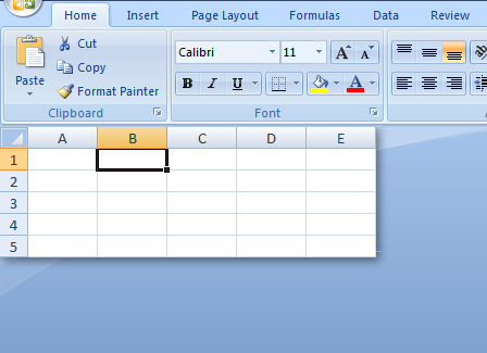
To restrict the work area,
- Select the first column you dont want to see (24th column) and press CTRL+SHIFT+RIGHT ARROW. Now Right click and select “Hide” option.
- Select the first row you dont want to see (45th row) and press CTRL+SHIFT+DOWN ARROW. Now right click and select “Hide” option.
Lock Formula Cells And Protect The Worksheet
Formulas are the most vulnerable part of an excel sheet. You accidentally edit something, say in payroll sparesheet, and you just gave 3200% bonus to someone in the organization. That is alright if that someone is a CEO of a bailed-out bank, but in all other cases, you end up spending a sweet afternoon trying to figure out what went wrong.

So, it is better to lock the workbook formulas and protect the worksheet so that no one accidentally erase the formulas or mess with them. To do this follow the steps in the illustration above.
You can use the same trick to lock the charts and other worksheet objects.
Freeze Panes So that Your boss Knows what she is Reading

Freeze panes is a very useful feature. It locks the important items on the top so even when you scroll down you still see them. (You can do the same for columns, thus seeing the first few column even when scrolling left).
Bonus tip: Use excel tables (new feature in Excel 2007) so that you dont need to freeze panes. Learn more.
Hide Un-necessary / Calculation Sheets
It is fairly common for excel workbooks to have tens worksheets, some with data, some with calculations, some with intermediate stuff and only one or two sheets with actual outcome (like a dashboard or a report).

There is no reason to think that all these worksheets should be visible all the time to the boss. While it makes sense to have the data and calculations visible so that someone can audit the worksheet, I am sure you dont want your boss to waster her time doing that. So here is a handy tip:
- Select all the worksheets other than the output sheets and hide them.
Hide Rows / Columns
If for some reason, hiding worksheets is not possible, you can still try hiding rows and columns. This is a very good way to prevent someone from accidentally messing a with a row of “really big and complicated formulas”.

Just select the rows / columns you want to hide and right click and select the “hide” option.
Include Cell – Comments / Help Messages
We all know bosses have a busy mind. They dont have time to remember (or know) every little thing. Heck, sometimes they dont even know what somethings are.

I suggest using cell comments and help messages to give right information / guidelines to the spreadsheet end user, like “enter your age in this cell”. They are easy to implement and totally non-intrusive.
- To include a cell comment, select the cell and press SHIFT+F2 and write the comment.
To include a cell message, select the cell, go to data validation, go to “input message” tab and type what you want.
Data Validations, Error Messages
Spreadsheets are complicated things that are carefully crafted with umpteen pre-conditions and assumptions. I am sure there is at least one excel file out there that will only work if a cat enters the input. But we are not talking about cats, the point is, it is important that right data is fed to the worksheet before the formulas (or charts or payroll macro etc.) can work. That is where data validation can help.

It is very easy to set up data validation in excel. Just select the cell and go to data validation (in Data ribbon / menu). There are several ways in which you can set up data validations,
- You can show an incell drop down box and ask users to pick from a list
- You can specify the type of data allowed (dates, times, numbers, text)
- You can specify the length of data
- You can specify the conditions on data (like between 2 numbers, less than a given date etc.)
- You can even use formulas to make your own data validations [example]
There are several examples of using data validation in this site. Go check.
Use Consistent Colors And Schemes
Anything looks better when it is consistent, even when it is internally screwed up. That same rule applies to excel workbooks as well. It will make your boss feel comfortable and relaxed to see an excel workbook with consistent colors and (simple) schemes.
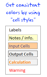
I suggest using excel cell styles to define the styles for your workbooks. This ensures consistency and you dont have to spend after hours formatting the worksheets. Read more about cell styles.
Name and Color Worksheet Tabs Appropriately
It doesnt matter if you have designed an awesome excel dashboard, your boss can be still pissed because the sheet name is “Sheet 69”. That brings us to the last and final point.

Use appropriate names (and may be tab colors) for the worksheet tabs. This makes the navigation easy and boss proof.
Learn how to color excel worksheet tabs.
Before Closing The Workbook, Select Cell A1 On The Correct Sheet
Just before you finally save the workbook and e-mail it to the boss, make sure you are on the right worksheet (ie the dashboard or the report) and selected cell A1. The ensures that when the boss opens the workbook, she sees the right tab with right information, not some calculations or formulas.
That is all, you have just learned a handful of trick to impress your boss.
Share your boss proofing tricks for excel
Got an awesome idea that has been working on your boss? Share it with us in comments. I love to hear your stories and how you are using excel to further your career.
Be awesome, Learn few more excel tricks:
We at PHD have a simple goal – “to make you awesome in excel and charting”. Here is a list of articles I recommend reading if you are new here or just wanted to be more.
- 15 fun and exciting excel tips – who say spreadsheets are boring?
- 15 Excel formulas beyond IF() and SUM()
- 15 Excel productivity tips that you dont know
- 10 things about Excel 2007 that you should know to work better
- More articles on excel productivity
Dilbert cartoon from Dilbert.com


70 Responses
Proper print settings on each sheet helps your boss to print the reports quickly without hastling you after printing irrelevant stuff.
It is highly relevant that you print your reports once before circulating it to your boss or other people.
Knowing that what your boss actully look at in the entire report can be very usefull. You can build a good summary of what your boss wants and put that as separate tab in the form of dashbord report, so that your boss does not peep into rest of your work and start pocking you with irrelevant stuff.
You can also put that Dashboard into the email summary and not trouble your boss to open your workbook. This is ultimate boss proof tip and I have been using this for long time now.
Thank you Chandoo. Great checklist to follow before delivering an excel spreadsheet to someone else. Some points you mention are seemingly so simple that we might overlook them – like selecting cell#A1, but they make a difference to the impression the spreadsheet creates at the recipient’s end.
Dear Chandoo,
Great tricks.
One trick I use (more and more) is to hide the sheet tabs and to hide the formulabar via the ‘tools’ ‘options’ and the ‘view’-tab.
Another trick is to limiting the scrolling area to hide all columms (or rows) until the end of the sheet. Select the column, press CTRL+SHIFT+RIGHT, right-click on the column and hide (also possible via VBA).
I was wondering though if ‘boss-proof’ is related to ‘excel-stupid-proof’?
Cheerio
Tom
Just wondering if the hiding formula bar really works when a recipient opens it whose “view-show-Formula Bar” is still checked…
It’s saved to the sheet I believe.
Absolutely agree with this post !!!
on the past months, after reading this blog, PTS’s and Debra’s Contextures, one of the things I’ve beggining to do as a best practice is to create all my spreadsheets with 3 tabs: data, summary and control, and this last one generally xlveryhidden, and sometimes the data one hidden as well.
And this restrictions are also being applied as best practice, and with a lot of benefits as you well mentioned. Furthermore, if combined with dynamic named ranges, formulae is more readable to users, and the WOW effect is often achieved when the question “How did you do that?” arises…..
Keep on the good posts !!!
Rgds,
Martin
Would you mind sharing an example of this technique?
Is there a way to keep the data in a seperate file rather than the same excel. This way you could keep presentation and data separate. But not sure how you would link up the two excel files
Yes, there is a way but it is not prefered.
I used this a coulple of times, (You need to code).
mail me if you need assistance with some sort
It entirely is possible. The problem comes though, when you share the spreadsheet.
If the recipient doesn’t have both files, or access to both, things break when the values try to refresh.
ey, why is the boss a she??
haha – welcome to the future. About time.
Chandoo, one more trick that we could use with the help of VBA, RT click on the View code of the particular sheet, in the properties table set the Visible status to 2-xlveryhidden, this ensures the sheet name does not show up even when the BOSS tries to unhide the sheet from the sheet >> unhide option. Dont forget to password protect the VBA (available under tools >> VBAProject properties.
Very good tips, although I have to say Chandoo, that your cats probably need to be spayed or neutered if they behave like that. =)
Good to see all these tips on a single “sheet”, and giving the name *boss proof*, and Dilbert was a great welcome 😀
The best way to “Boss Proof” (and “Self Proof”!!) a spreadsheet is to keep back ups. I use a macro that saves the last 3 significant versions of the spreadsheet all with a date stamp included in the file name.
To quickly select cell A1 on all sheet, use CTRL-Page UP or CTRL-Page down to navigate between sheets and CTRL-Home to select cell A1 (if you have frozen pane, it will select the top left cell of the section below).
Great list. And I follow every single item… I also use a consistent background color for input cells in every report/dashboard. And I use a little VBA to identify the user and change the report accordingly (selecting the right market, for example).
Chandoo, Nice post. I like to use the hidden Paste Picture Link option. Keep the original report you want displayed on a hidden sheet and only show the boss the report picture. Also great to watch the confusion when boss trying to select cells is worth the effort!
I usually save as PDF if there’s no interactivity in the report. That way nothing can go wrong 🙂
PDFs work a dream for me too and saves the boss’s EA from telling me all the time that she can’t print my work!!
@All.. thanks a ton for sharing your ideas. I am thinking of writing a part 2 of this post explaining some of your ideas in detail.
@Bazlina … I will make sure the boss is a HE in the next post 🙂
“10 Tips to Make Better and Boss-proof Excel Spreadsheets”…
Unless of course your Boss reads PHD !
Great article with one glaring error.
If (like me) the majority of your spreadsheet errors are *caused* by cats, adding more cats is just going to increase the problem.
@Hui you always have a boss, even if you are boss. If you dont have a boss, then may be a cat or even a dog.
@Debra: hmm… Are you sure the cats are not after the mouse? Go learn some keyboard shortcuts.. now 😛
Great Web Site. I’ve done almost all the above in trying to build my application and it’s taken me hours and hours reading my “dummies ” book. Thank you for all this information.
Is there a formula I can use that will automatically return to “A1” cell should an associate use the 10 page spreadsheet I have?
Is there a way to set an expiration date on my workbook so that beynd that date no one will get beyond the cover page?
Paul, in all my “user facing” workbooks (those that I distribute) I create a named range called “Home” on the worksheet(s) that are most likely to be used. Then I write a little VBA that selects the Home range whenever that worksheet is activated or on other triggers depending on the context of the sheet. This is more appropriate for the dashboard tabs or summary tabs my job requires.
But I usually set this functionality up early on in the design process so I can take advantage of it as well. I will sometimes assign a keystroke to the GoHome macro.
I’m in the marketing department (aka the picture department) and have to say that the macros/Excel sheets from our controlling department are the worst! They come to me to sort out the mess!!
@Peter: You can try creating a table of contents and then place it on each and every sheet so that user can jump to anywhere from anywhere. Here is a tutorial to help you get started.
Also, You can prevent users from accessing the workbook after a certain date using macros. But users can certainly by pass it by disallowing macros on that workbook.
@Jimmy: Wow… (just kidding) Welcome 🙂
I was recently given a spreadsheet to improve upon.
One of the “boss-proof” actions that the previous author had used was to use data validation instead of protecting the sheet to ward off people changing formulas.
After entering a formula or value into a cell, use data validation to only allow, in this spreadsheet, whole numbers between 9999999 to 99999999.
It’s a bit of a pain to actually correct stuff instead of just unprotecting a sheet, but for those that know how to unprotect a sheet, it’s a definite way to keep them from fooling with formulas.
Puchu,
We would love to see “Print” in your links section.
It helps us taking prints as neat as your posts 🙂
Chandoo,
I’ve emailed you a couple of times looking for avenues I need to try to put my workbook on the Internet.
I notice you use PremiumThemes for your Web Site…You must feel good about their service. Do you think PremiumThemes might be an option for me?
Paul
Instead of :
Now Right click and select “Hide” option.
Shortcut can be used : Ctrl+0 (to hide)..
sir i wanted to know,how to hide cells or tab without hiding rows and columns? PLZ TELL ME
Hi Chandoo!
Great tips! Im researching on an excel project now that you can create to “lighten” the size without sacrificing the data inside..
We usually encounter problems with the data, excel file is shared, in a network folder.. and there are 11 people that enters their own productivity in each tab.. however, there comes a time (uncertain) where some of the data they enter either gets deleted or changes value.. could this be a file size problem? are there other ways to create this file that will decrease data inconsistencies?
thanks!
You will find another quick and easy technique here:
http://www.onsitetrainingcourses.com.au/main/page_blog_hiding_most_excel_rows_and_columns.html
Save what you want the boss to see as a PDF. Absolutely foolproof and no cats hurt in the process.
I really enjoyed allot of the tips on here, especially the one on comments on cells. That will come in handy on allot of our projects. I would also like to share on on my little tricks. I am constantly working on several different reports with several different systems and in doing so I am constantly running in problems and my way out of them is simply calling <a href”http://www.reportingguru.com/”> Reporting Guru </a> and telling exactly what I’m going through and they can tell me exactly how to get out.
One of the things I’ve found to boss proof my worksheets are a few simple VBA scripts to automatically protect the workbook/worksheets, and direct them to the “Quick Look” dashboard page, I hide all of the raw data sheets before saving. The script looks like this:
Private Sub Workbook_Open()
Sheets(“Summary”).Protect Password:=”password”
Sheets(“Labor Cost by Site”).Protect Password:=”password”, AllowUsingPivotTables: =true
Sheets(“Labor Cost by month”).Protect Password:=”password”
Sheets(“Quick Look”).Protect Password:=”password”
Sheets(“Quick look”).Activate
ActiveWorkbook.Protect Password:=”password”, Structure:=True, Windows:=False
End Sub
I also have a pivot that contains labor cost data which cannot be refreshed while the worksheet is locked.
Private Sub Worksheet_Activate()
Sheets(“labor cost by site”).Unprotect Password = “password”
Set pvttable = Worksheets(“labor cost by site”).Range(“a1”).PivotTable
pvttable.RefreshTable
Sheets(“labor cost by site”).Protect Password = “password”, AllowUsingPivotTables:=True
End Sub
OPPAN GANGAM STYLE!
good
Your post are always with something creative , thanks for sharing this information , your post are worth reading and implementing 🙂 great job
Hi,
I will try to learn every point slowly !
Shokran Chandoo.
Best boss Proofing of sheets is useing indirect(address 😛 this prevents most smartass bossess from doing any actual changes cus the formula will be long and hard to understand for any bystanders..
Also putting the actual calculations on a different sheet can make a sheet bulletproof from bosses.. especialy if you put them in the Very hidden so when the boss learns how to unhide sheets he wont simply find them.
One thing iv also learned is that most bosses is scared of macros that gives “virus” warnings before beeing run 😛 That include the default warning from Excel…
Long formulas or work arounds is best way to go.
What’s the best way to amalgamate two existing excel spreadsheets into one?
Two teams use the same format spreadsheets with individual data split into calendar months and I want to make them one without manually entering the data.
Alt + D + D + N
Write a query and viola, Two sheets into one.
Changing the properties of the file to read-only . (While the file is closed, right click on the file and check the read-only box.)
This allows my boss(es) to access the file — even change it — without being able to save their changes. If a boss likes his ‘new’ version, he can save it with a different file name.
But now — how to prevent the boss from deleting the file altogether? Or deleting the whole network?
Hey man.
Think you can go as easy as to make a shortcut that links to your read only document. Then the boss wont know of the root document. He can figure it out but lets face it. He is a boss and 70% if them wont know squat
Instead of “Hiding” rows & columns, I find “Grouping” works best as its very easy to quickly see if a worksheet has hidden rows/columns. Sometimes hiding a random row/column is not easily noticed and can create issues.
I have one xl sheet with different dates in many columns and one raw’s. I want to send this data to another xl sheets for each date. if somebody can help me will be great.
Dear Samantha,
Check out the website of Ron de Bruin. He has a great set of macro’s and free add-in that can help you with this issue.
http://rondebruin.nl/win/s3/win006.htm
Tom
Hello, I have just found out that I made a mistake in my spreadsheet: I had a column of negative numbers, but one of them was positive (while it should have been negative). Is there a formula/system to avoid this?
Thanks.
Mariateresa
Yes, data validation. Values you denote would be between -1 and -999,999,999.
Hi,
Hiding any worksheet can be unhidden and messed around easily. I change the visibility in visual basic from -xlSheetVisible to -xlSheetVeryHidden. By this, even if you right click on sheets, you will be unable to find the hidden sheets.
Cool? I think so…
Very informative, Thanks
Is there a way to lock cells in an already protected worksheet.
(Thus the entire worksheet is protected, then the entire office can open it as read only but only a few users have the password to edit the file)
I would like an additional password or prompt box so these few users don’t accidentally change formulas.
Itss such as you learn my thoughts! You appear too understand
a lot abnout this, like you wrote thee e-book in it
or something. I fel that you just could do with some percent to presseure the message house a little bit,
but insatead off that, this iis wondeerful blog.
An excellent read. I’ll definitely be back.
It is in reality a nice and helpful piece of info.
I am happy that you just shared this useful info with
us. Please keep us up to date like this. Thank
you for sharing.
I laughed out loud reading the 2nd solution about moving to marketing department and making ppts.
I’ve been using “technical” sheets for a long time already and depending on the audience it is hidden or not. I’m currently in my NO VBA mindset, so the very hidden option is no longer. Using sheets names like: TechnicalCodes; ExplicitVariables;SetUp; HeavyCalc seem to work to my experience as they send along a message “Don’ t you mess-up here, you fool!”. A “Read This” section or sheet however does not work!
Reading stuff on this site has helped me develop a good habit of using colors and themes to assist the end user in being well-behaved. In my book the best advise here, because it is about the user experience and not only about protection your own work.
For dashboards I get rid of tabs and scroll bars. Besides 2 exceptions, I need to come across a manager who can turn them on again without my help.
Seems that I forgot about protecting cells, sheets and workbooks altogether. Damn!
Thanks for the informative article Chandoo, I’ve been struggling with Excel lately. It’s a powerful tool, but hard to learn for me.
Thanks Chandoo for sharing these excel sheet tips it helps me a lot to understand excel more.
Nice roundup, Chandoo! Here’s one more I thought would be relevant:
For Excel 2013+, you can hide the ribbon, as shown in this animated gif: https://gridmaster.io/tips/hide-ribbon-excel-space
This will simplify the interface, making it less likely for people to accidentally make changes. 🙂
THANK YOU SIR
I’m better at Power BI thanks to you!